Diabetic Kidney Disease Prediction Using Hybrid Deep Learning Model

Among the many long-term consequences of diabetes, chronic kidney disease (CKD) is the most expensive and causes significant disruption to daily life [1]. Negative health consequences that may arise from CKD include frailty, decreased quality of life, renal illness, increasing end-organ damage, and early mortality [2]. Indeed, the higher mortality related to type 1 and type 2 diabetes is primarily limited to people with CKD. Consequently, a vital goal of diabetes care is the prevention and management of CKD. About half of people with type II diabetes and one-third of those with type I diabetes will have CKD [3]. This condition is clinically described by either impaired kidney function or elevated levels of albumin in the urine, or both. The exact proportion of individuals who might be diagnosed with CKD due to their diabetes is unknown. Severe kidney damage, dyslipidemia, glomerular atherosclerosis, weight gain, intrarenal vascular disease, renal ischemia, high blood pressure, and age-related nephron loss are factors that might contribute to renal dysfunction [4]. Therefore, it is hard to identify 'diabetic kidney disease' (DKD) or 'diabetic nephropathy' in epidemiological or clinical settings, especially among patients with type 2 diabetes [5]. It is better to seek out individuals who have both diabetes and CKD and to employ measures for comprehensive renoprotection. Despite its high prevalence, mortality rates, and treatment expenses, DKD is mostly unrecognized and untreated, despite being a significant microvascular complication of diabetes mellitus.

Microalbuminuria, an increase in urine albumin excretion, is the first symptom of DKD [6]. It is followed by large albuminuria and a quick decrease in renal function [7]. The accepted opinion holds that proteinuria is the first sign of deteriorating renal function. However, this hypothesis has been called into question because many patients have shown improvements in their albumin excretion rates, either on their own or after receiving comprehensive risk management. Since DKD is typically mild when it first appears, the value of microalbuminuria as a conventional sign of the disease and the best time to take action are both questioned. Although renal biopsy may differentiate DKD from normal kidney disease, there is currently no gold standard for predicting DKD development [8]. Not everyone follows the recommendation to increase screening frequency, which can lead to delayed diagnoses. To improve survival rates and quality of life for diabetes patients and decrease the occurrence of cardiovascular events, it is crucial to prevent, diagnose, and treat DKD as soon as possible [9, 10]. There is an immediate need for a clinical instrument that is both simple and easy to use for evaluating DKD in everyday practice.

To monitor and diagnose DKD, it is crucial to develop an automated system that relies on simple predictors, such as clinical data. Many diseases are predicted using DL algorithms because of their superior performance on large datasets with high-dimensional features. Research on DKD prediction models has mostly relied on a single classifier and employed relatively limited sample sets. When there are too many variables and samples, models face the risk of underfitting or overfitting, which diminishes their effectiveness. To improve the predictive reliability and accuracy of these models, we used hybrid DL models to classify DKD from normal samples.

2.    Literature Survey

The recent work on kidney disease prediction using ML and DL models is discussed in this section. The study [11] aims to determine the optimal classification approach for DKD prediction by comparing the results of various methods applied to a DKD dataset using the WEKA ML tool. Nine different classification algorithms were tested on a DKD dataset with 18 attributes and 410 instances. Data preparation included tenfold cross-validation. Performance was assessed using metrics such as execution time, accuracy, and error rate. The outcome shows that the best performing algorithms were random tree classification, instance-based learning with k-nearest neighbors (IBK), among others. Research [12] focuses on the development of a predictive model for CKD. It highlights the common use of ML algorithms in medicine for disease prediction and classification. Bias in medical records was addressed by analyzing a dataset on CKD with 25 features from the University of California (UCI) ML repository, using several ML models. The bagging ensemble approach was employed to enhance model performance. The decision tree classifier yielded the best results when applied to the chronic renal illness dataset's clusters.

The study [13] introduces a novel DL model for early CKD diagnosis and prediction. The research aims to develop a DL network and compare it with other advanced ML techniques. Missing database variables were imputed with the average of relevant attributes. After parameter tuning and multiple trials, the neural network's optimal parameters were determined. Recursive Feature Elimination (RFE) was used to identify significant traits, which were then fed into ML models for prediction. The proposed Deep Neural Network (DNN) performs better than the other models in terms of accuracy. A study [14] investigates whether ML can predict which CKD patients will progress to severe kidney disease. Data were collected from a CKD cohort monitored over time. Predictor factors included blood test results and baseline features. Multiple imputation was used to handle missing data. Five ML algorithms were trained and evaluated using a five-fold cross-validation approach. Performance was compared to the Kidney Failure Risk Equation (KFRE). The ML models (naïve Bayes, logistic regression, and random forest) demonstrated comparable predictability and higher sensitivity than KFRE. The study showed that ML can effectively assess CKD prognosis using easily available features.

The paper [15] aims to assist medical practitioners in diagnosing CKD patients using ML technologies. The CKD dataset from the UCI repository was analyzed with various ML algorithms, including K-nearest neighbor (KNN), support vector machine (SVM), and DNN. Different methodologies were employed to impute missing values, considering the correlations of features. Hyperparameters of each method were fine-tuned, and the performance was evaluated using various criteria. The findings indicated that DNN outperformed the existing methods in accuracy. In the study [16], researchers explored the use of various ML methods for DKD prediction. Combining these classification approaches with cloud computing services significantly improved treatment decisions for DKD patients. Classifiers were trained to detect CKD cases using clinical features from the UCI Repository. While single clinical features yielded the best performance with SVM, RF, and KNN classifiers, the highest accuracy was achieved by combining clinical features using DL and RF.

3.    Materials and Methods

The method used to predict DKD from the clinical data is discussed in this section. The process starts with data collection, followed by data processing, feature selection, model construction, training, validation, and testing. Finally, the best model is identified using performance metrics.

• 3.1    Data Acquisition

  The dataset used in this study was obtained from a publicly available repository on Kaggle. The dataset consists of 1000 samples, with 503 DKD instances and 497 normal instances, resulting in a near-balanced class distribution that enables fair evaluation of classification performance without bias toward a dominant class. The features included in the dataset are patient_id, age, gender, medical_history, blood_pressure, blood_sugar, cholesterol, creatinine, and GFR. The dataset consists of anonymized clinical records related to kidney disease and does not contain any personally identifiable information. As the dataset is publicly accessible and anonymized, the use of this dataset does not require ethical approval or informed consent. These features provide a comprehensive set of clinical parameters that are

• 3.2    Data Processing

relevant for predicting DKD. In this dataset, gender and medical_history are categorical variables and the other features are numerical, representing continuous values that quantify various aspects of the patient's health. Accordingly, the experimental setup and results presented in this study are fully reproducible.

Before the ML classifier, data must undergo data preparation, which involves cleaning and transforming the raw data to ensure it is suitable for analysis [17]. Common data preprocessing techniques include handling missing data, outliers, duplicates, data normalization, and encoding methods used in this research.

Missing Data: Missing data can lead to unreliable statistical findings, distortions, and poor decisions, significantly affecting the integrity and applicability of datasets [18]. Classification errors can arise when data contains missing values. Imputation was employed to fill the missing values [19]. When data is missing from a dataset, imputation can fill in the gaps while preserving the majority of the data. These strategies are necessary because regularly removing data from the dataset is impractical and can significantly reduce its size, raising concerns about bias and leading to inaccurate analysis. Another factor compromising classifier accuracy is data duplication. Identical instances were identified and removed.

Outlier: An outlier is a data point that deviates considerably from the rest of the observations in a dataset [20]. Outliers, which can occur for a variety of reasons, can have a disproportionate impact on statistical analyses and ML models if they are not managed properly. In statistics [21], the z-score is a crucial measure to identify how far a data point is from the mean and the magnitude of this difference. Equation (1) provides the formula for calculating the z-score.

х—у.

ст

Normalization: Data normalization is the process of adjusting feature values so that they are on a similar statistical scale, ensuring they have equal relevance [22]. DL models perform better when data is normalized, therefore all features are normalized before classification in this research. The Min-Max normalization [23] technique is employed.

Encoding: Gender, medical history, and the target column data in the collected dataset are categorical. This study uses one-hot encoding [24], which represents categorical data using a vector where only one element is set to one while all other elements are zero.

To prevent any form of data leakage, all preprocessing steps, including normalization, encoding, and feature selection, were performed using parameters derived exclusively from the training dataset. The same preprocessing transformations were subsequently applied to the validation and test sets without recalculating any statistics. The test data were strictly isolated and were not used at any stage of model training, feature selection, or hyperparameter tuning.

• 3.3    Features Selection

  

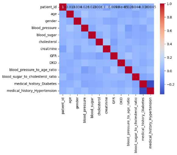
  Fig. 1. Correlation Matrix of DKD Dataset Features

  
  

In ML analysis, feature selection plays a crucial role. It involves selecting relevant features from a larger pool of available ones. The primary objective of feature selection is to find and retain the most informative features while disregarding unnecessary ones [25]. By eliminating redundant information and focusing on essential data, models can be enhanced. Feature selection strategies also lead to reduced data dimensionality and improved model performance. The correlation matrix serves as a tool for feature selection [26]. The correlation matrix measures the linear relationship between pairs of features in a dataset, indicating both the strength and direction of their relationship. A correlation value of 1, 0, and -1 represents the strong positive, no, and strong negative correlation. Fig. 1 illustrates the correlation matrix of the dataset.

Based on the correlation values, the important features are selected while the remaining features are dropped. This step ensures that the models are trained using only the most relevant features, which helps in improving their performance and reducing complexity. The statistical analysis of the selected features is conducted using various visualization plots. Figs. 2-4 illustrate the results of this analysis through different types of plots: histograms, box plots, and scatter plots.

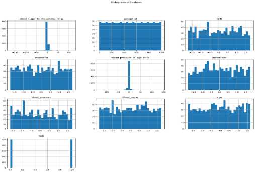
Fig. 2. Statistical Analysis of Selected Features Using Histogram

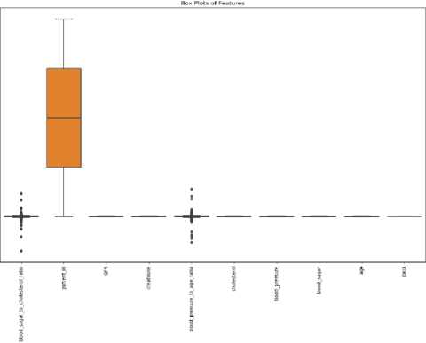
Fig. 3. Statistical Analysis of Selected Features Using Box Plot

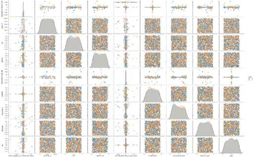
Fig. 4. Statistical Analysis of Selected Features Using Scatter Plot

During the feature selection process, non-informative and identifier attributes were excluded to prevent data leakage. In particular, the patient_id attribute was used solely for record identification and was removed prior to model training and evaluation. Correlation-based feature selection was applied exclusively to clinically relevant numerical features, and the target variable was not included in the correlation computation. This ensured that the selected feature set did not introduce any form of information leakage into the learning process.

• 3.4    CNN

CNNs are primarily concerned with learning the spatial hierarchies of features, which range from basic to advanced patterns [27]. Training a CNN involves identifying significant patterns in incoming data. In this process, learnable filters are applied to a set of convolutional feature extractors in the early layers. Each CNN layer generates its own feature map using convolutional kernels. To create a feature map, all the input spatial locations share the same kernel. Once the Convolutional Layer (CL) and Pooling Layers (PL) are completely constructed, the Fully Connected Layers (FCL) are employed to finish the classification. In CNNs, Equation (2) illustrates the process of convolution on input feature maps and CLs:

^{ℎ (}„) _=∑Lx ℎ ⁽ г¹ ) _⊗ w⁽”) ₊ b ⁽" ⁾                                    (2)

The outcome of the jth feature map in the n^th hidden layer (HL) is given by ℎ ^{( )} , ⨂ indicating 2D convolution. In contrast, ℎ ^{(   )} indicates the k^th channel in the ( n -1) th HL, w ^{( )} indicates the weight of the n^th layer, and

^{( )} indicates the corresponding bias. To minimize the feature dimensions, an extra layer is inserted into the CLs, resulting in a huge number of feature maps. A PL is a method for reducing the computational costs and overfitting concerns involved with network training.

To complete CNN training, an iterative technique is used to alternate between feed-forward and backpropagation [28]. Iterative backpropagation includes changing the convolutional filters and FCL. The aim is to minimize the total average loss E between actual and model outputs. The Equation (3) shows the loss function.

E _{=  ∑} ^ ^∑ к=1У ̂ ( ) _log( У, ⁽ к ⁾ )                                   (3)

The true label is represented by ̂ ^{( )} , while the model outcome of the i^th input in the k^th class is denoted by y_{ . Additionally, с is the total neurons in the final layer, while m represents the training inputs.

Convolution Layer: Convolution operations give rise to the moniker CNN. The Convolutional Layer (CL) is a crucial component of the CNN architecture because it is responsible for feature extraction [29]. Typically, the layer includes an activation function and a convolution operation, both of which are nonlinear. To strengthen the spatial relationship between pixels, convolution processes use learnable characteristics and a filter known as a kernel [30]. During CNN training, automatic adjustments to the kernel values are made to enhance the model's ability to learn new input features. The feature map size is calculated by the dimension of stride, filters, and padding.

Pooling Layer: In most circumstances, the Pooling Layer's (PL) is used to minimize the feature map dimensions, making them more insensitive to small distortions and motions [31]. This also reduces the number of learnable parameters in the subsequent layers. Interestingly, none of the PLs have any learnable parameters. For this reason, the PL's capacity to undersample features is critical for lowering network complexity and preventing overfitting. To represent the output of an entire region, Max Pooling is employed and it takes the maximum value of all neurons in that region which is represented in Equation (4):

=max i ∈ ℛ Xi                                            (4)

The PL usually comes after the CL. Its primary goals are minimizing parameters to prevent overfitting, improving training speed, and reducing the feature matrix dimension.

Fully Connected Layers: All neurons in one layer are considered "fully connected" (FC) if they are linked to all the neurons in the next layer [32]. Flattening, or presenting the output feature map as a 1-dimensional set of numbers coupled to one or more FCLs, sometimes known as dense layers, is common practice for the final CL or PL. Each input in these layers is paired with an output based on a learnable weight. FCLs can be used for feature mapping once the features have been downsampled in the PL and extracted in the CLs. The network's final outputs, which are the probabilities for each class, can then be determined in this manner. In most cases, a SoftMax classifier follows the FCL. In this example, n neurons are utilized to represent the number of classes.

Recent research combining CNNs and recurrent neural networks (RNNs) has yielded remarkable results in a variety of disciplines [33]. To improve model learning efficiency, CNNs reduce the number of parameters by sharing their weights. Furthermore, the LSTM model addresses the RNN's long-standing concerns with gradient explosion and vanishing gradients.

Fig. 5 demonstrates the comprehensive structure of the CNN-LSTM network, which combines the advantages of both 1D-CNN and LSTM algorithms. This novel technique integrates two distinct learners: the first concentrates on local abstraction, capturing the spatial aspects of the input, while the second focuses on sequence modeling to comprehend temporal dynamics. The CNN serves as a feature extractor, recognizing and encoding the most important properties of the input data. After the CNN has learned the spatial features, the LSTM takes over to extract essential location-based information, leveraging its capacity to detect long-range dependencies in the data. This hybrid design enables the CNN-LSTM model to accurately capture the basic features of the data while enhancing its ability to derive significant insights, making it especially suitable for improving accuracy. By combining these models, the system improves its ability to distinguish between different types of data, resulting in greater adaptability to diverse and complex patterns. The model's strength lies in its capacity to extract hidden features from the data, enhancing decisionmaking capabilities and boosting overall performance across datasets. Algorithm 1 defines the pseudo-code for the CNN-LSTM model, whereas the preceding sub-section discusses the functionality of the CNN. This hybrid learning framework offers an advanced method for concurrently processing and evaluating the data, pushing the capabilities of traditional CNN and LSTM architectures.

Both CNN and CNN-LSTM models were trained using identical hyperparameters, which are summarized in Table 1.

Table 1. Hyperparameters Used for CNN and CNN-LSTM Models

Hyperparameter	CNN	CNN-LSTM
Input shape	(9, 1)	(9, 1)
Number of convolution layers	2	2
Number of filters	32, 64	32, 64
Kernel size	3	3
Activation function	ReLU	ReLU
Pooling type	Max pooling	Max pooling
Pool size	2	2
LSTM units	–	50
Fully connected layers	1	1
Optimizer	Adam	Adam
Learning rate	0.001	0.001
Loss function	Binary cross-entropy	Binary cross-entropy
Batch size	32	32
Number of epochs	50	50

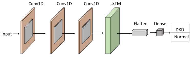
Fig. 5. Architecture of the Proposed CNN-LSTM Model

Although the clinical dataset used in this study is tabular in nature, the CNN-LSTM architecture is employed to effectively capture complex feature interactions and dependencies. The selected clinical features are reshaped into a one-dimensional input tensor to enable convolutional operations. The CNN component acts as an automatic feature extractor, learning local patterns and interactions among clinical variables, while the LSTM component models interfeature dependencies by retaining contextual relationships across the feature sequence. This hybrid design allows the model to leverage both spatial feature abstraction and dependency learning, making it suitable for structured clinical data despite the absence of explicit temporal information.

LSTM: A recurrent neural network model known as LSTM tackles the age-old problems of RNN models, such as gradient explosion and vanishing gradients [34, 35]. Equation (7) expresses the LSTM model's hidden activation for each data input ^xt . The next step is to input and use all of the data for forecast purposes. The LSTM unit, which accepts the current state's input ^xt and the acquired information ℎt-1 as inputs, is in charge of defining the transformation relation ℎJ of the hidden representation in the LSTM model. Thus, the LSTM network processes data inputs and passes on inherited information to the next level [36].

Algorithm 1: CNN-LSTM

Initialize model parameters

CNN: ( w ⁽" ) _, Ъ ^{( n}i ⁾ ), LSTM: ( w_c , w_f , Wt , w₀ , be , bf , bi , b₀ ), FCL: ( WpeL , bpCL )

For CL:

For feature map j in the current layer: ℎ ^{( )} =0

For feature map к in the previous layer: ℎ ⁽ n ) _=∑ k-i ℎ^{( П 1} )_⨂ W ⁽ ” ) ₊ b ⁽ 7)

Apply activation function ℎ⁽ ” ) ₌ ReLU (ℎ ⁽ n ) ₎

For the PL:

For the region in the feature map: Yt = ∈ ℜ ^xl

Flatten the output of the last CNN layer

For each time step :

Calculate candidate memory ^̃=    ℎ( W_c ․[ℎ t-1 , Xj]+ be )

Calculate forget gate ft =( Wf .[ℎ t-1 , ^xt ]+ bf )

Calculate input gate f =( Wi .[ℎt-1, ^xt ]+ bi )

Calculate output gate °t =( W_o .[ℎt-1, ^xt ]+ b₀ )

Update cell state =   ∗     +   ∗ ̃

Update hidden state ℎJ=   ∗ tan ℎ( C^ )

FCL for final output: y_} ⁽ к ) ₌ ReLU ( WpQL * ℎ_t+ bpCL )

For each class к :  Probability У1 ⁽ к ⁾ = SoftMax( У1 ⁽ к ⁾ )

Loss calculation using cross-entropy: E _{=  ∑} i=i ∑ k=i ̂ ^{( )} log ( У () )

Update weights and biases to minimize loss E

Equation (6) is used to compute the memory cell C^ , which is present in each LSTM cell. Using Equation (5), each LSTM generates a new potential ̃^ to replace C^ . This ̃^ serves as a memory to help the hidden unit recall past information. The LSTM's memory unit is the most critical component for preventing gradient explosion and vanishing gradients.

̃ = tanh(Wc⋅[ℎt-1, xt]+be)(5)

=  ∗     +  ∗ ̃(6)

ℎt=   ∗ tanh(ct)(7)

The LSTM subsequently creates three gates: forget ( ft ), update ( it ), and output ( °t ).

h =σ(Wt⋅[ℎt-1, xt]+bi)(8)

ot =σ(Wo⋅[ℎt-1, xt]+b0)(9)

ot =σ(Wo⋅[ℎ  , xt]+bo)(10)

Where, W_c , W_L , W^ , and W_o represents the weight parameters, and b_c , bi , bf , and b₀ represents the bias parameters. c^ is produced by combining ℎ t-1 (previous hidden state), ℎJ (current hidden state), and C^_ .

4.    Results and Discussion

The DKD and normal data were collected and processed, including the elimination of outliers, handling of missing data, removal of duplicates, data normalization, and encoding. From the processed data, important features were selected using a correlation matrix. The data were then split into training, validation, and test sets with proportions of 70%, 10%, and 20%, respectively. The data splitting process was performed using a stratified sampling strategy to ensure that the class distribution of DKD and normal instances was preserved across the training, validation, and test sets. A hold-out validation strategy with a 70/10/20 split was employed in this study to evaluate model performance. While this approach provides an initial assessment of the proposed model, it does not capture performance variability across multiple data partitions. Stratified k-fold cross-validation is recognized as a more robust evaluation strategy, particularly for limited datasets, and will be incorporated in future work to further assess the stability and generalizability of the proposed model. The selected features and targets from the training samples were fed into CNN and hybrid CNN-LSTM models. Both models were evaluated using Accuracy and loss metrics during the training and validation phases.

The loss and accuracy plots for the CNN model on training and validation data are shown in Fig. 6 and Fig. 7. The loss score reached 0.1 in both phases, with a maximum Accuracy of 96% during training and 95% during validation. The loss and accuracy plots for the CNN-LSTM model on training and validation data are depicted in Fig. 8 and Fig. 9. The loss score reached less than 0.1 in both phases, and the maximum Accuracy attained was 99% for both the training and validation phases.

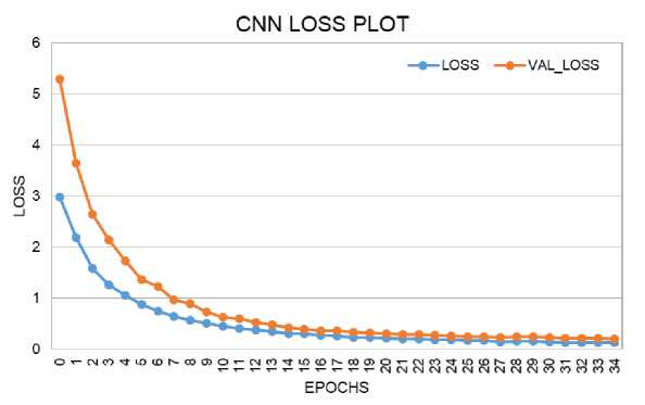
Fig. 6. Loss Performance Curve of CNN Model During Training and Validation

Fig. 7. Accuracy Performance Curve of CNN Model During Training and Validation

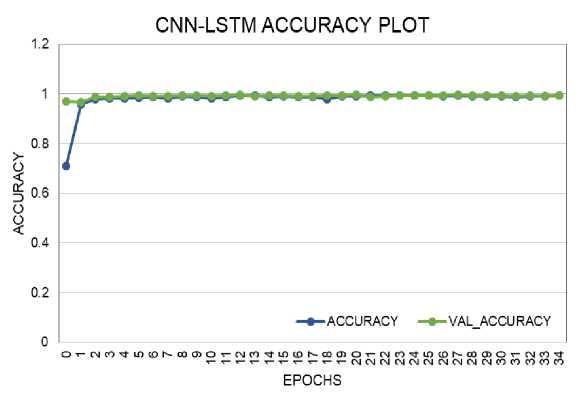
Fig. 8. Accuracy Performance Curve of CNN-LSTM Model During Training and Validation

CNN-LSTM LOSS PLOT

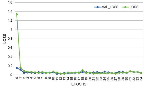
Fig. 9. Loss Performance Curve of CNN-LSTM Model During Training and Validation

After training both the CNN and CNN-LSTM models, the remaining 20% of the data was used to test the models. The confusion matrix for the CNN model's DKD prediction is presented in Fig. 10. The True Positive (TP) and True Negative (TN) values were 96 and 97, respectively. The False Positive (FP) and False Negative (FN) values were 5 and 2, respectively. The confusion matrix for the CNN-LSTM model's DKD prediction is shown in Fig. 11, with TP and TN values of 98 and 100, respectively, and FP and FN values of 1 and 1.

	Predicted	Predicted
	DKD	Normal
Actual DKD	96	2
Actual Normal	5            97

Fig. 10. Confusion Matrix of CNN Model for DKD Prediction

The confusion matrix of the CNN-LSTM model on DKD prediction is given in Fig. 11. The TP and TN values attained by the CNN-LSTM model are 98 and 100. The FP and FN scores of the CNN model are 1 and 1.

Predicted               Predicted

	DKD	Normal
Actual DKD	98	1
Actual Normal	1	100

Fig. 11. Confusion Matrix of CNN-LSTM Model for DKD Prediction

Based on the confusion matrix values (TP, TN, FP, and FN), performance measures were calculated. The performance metrics used were Accuracy, Sensitivity, Specificity, Precision, and F1-score. The Accuracy of the CNN and CNN-LSTM models were 96.5% and 99%, respectively. The sensitivity, specificity, precision, and F1-score for the CNN model were 95.1%, 97.96%, 95.05%, and 96.48%, respectively. For the CNN-LSTM model, these metrics were 99.01%, 98.99%, 98.99%, and 98.99%, respectively. The performance comparison of the CNN and CNN-LSTM models is given in Fig. 12. This comparison plot highlights the superior performance of the CNN-LSTM model in predicting DKD. The ROC plots, which also validate model performance, are shown in Fig. 13 and Fig. 14. The ROC values for the CNN and CNN-LSTM models were 97.62% and 98%, respectively.

Even though the proposed CNN-LSTM model achieved high performance metrics, including an Accuracy of 99%, these results should be interpreted with caution. The evaluation was conducted on a relatively small test set, and the near-perfect performance may partially reflect the balanced nature of the dataset and the effectiveness of feature preprocessing and selection. High accuracy values on limited datasets may also indicate a potential risk of overfitting, despite the use of validation data. Therefore, the reported results primarily demonstrate the comparative effectiveness of the CNN-LSTM model over the CNN baseline within the given experimental setting

PERFORMANCE COMPARISON OF DKD PREDICTION USING DL

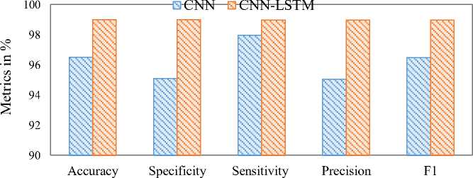
Fig. 12. Performance Comparison of CNN and CNN-LSTM Models

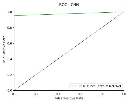
Fig. 13. ROC Curve of CNN Model for DKD Prediction

However, a formal ablation study isolating each architectural component was not conducted in this work, the comparative evaluation between the CNN and CNN-LSTM models provides insight into the contribution of the LSTM layer. The observed performance improvement of the CNN-LSTM model over the standalone CNN indicates that incorporating dependency modeling enhances predictive capability. A comprehensive ablation study analyzing the individual and combined effects of architectural components will be explored in future work to further quantify their contributions.

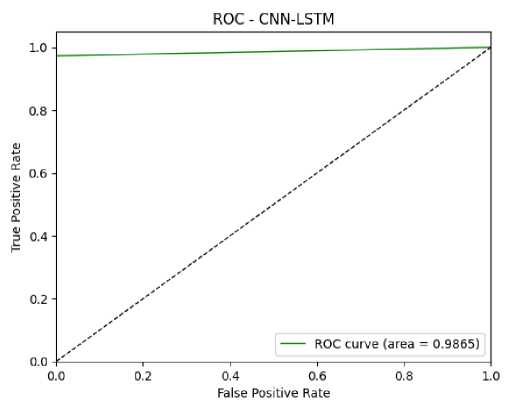
Fig. 14. ROC Curve of CNN-LSTM Model for DKD Prediction

In Table 2, the performance of the proposed CNN-LSTM model for DKD prediction is compared with recent work. In most of the studies, metrics like specificity and ROC are not considered; they focus only on accuracy, precision, sensitivity, and F1-score. The comparison shows that the proposed model achieves a higher Accuracy of 99% compared to recent research models like XGBoost, Random Forest, optimized CNN, CNN, and Extra Trees.

Table 2. Comparison of the proposed model with previous research

Ref	Ours	[37]	[38]	[39]	[40]	[41]
Model	CNN-LSTM	XGBoost	Random Forest	Optimized CNN	CNN	Extra tree
Accuracy (%)	99	98.3	96	98.75	97.16	98
Specificity (%)	99.01	-	-	-	-	-
Sensitivity (%)	98.99	98	97	98	97.18	98
Precision (%)	98.99	98	97	96.55	97.24	99
F1-score (%)	98.99	98	97	99	97.17	99
ROC (%)	98.65	-	-	-	97.62	-

In this study, comparative analysis primarily focuses on tree-based ensemble methods and deep learning models, as these approaches have demonstrated strong performance on structured clinical datasets in prior studies. Classical machine learning classifiers such as Logistic Regression, Support Vector Machines, and k-Nearest Neighbors were not included as baselines in the current implementation. This choice was made to emphasize comparison with more competitive and commonly adopted models for medical decision-support systems. Nonetheless, the inclusion of traditional machine learning baselines represents an important direction for future work to provide a more comprehensive comparative evaluation.

5.    Conclusion

This study successfully implements a hybrid CNN-LSTM model for predicting Diabetic Kidney Disease (DKD) using clinical data. The research begins with meticulous data collection and preprocessing to eliminate outliers and refine the dataset. Feature selection is carried out based on a correlation matrix. Both CNN and CNN-LSTM deep learning models are trained and evaluated using key performance metrics. The CNN-LSTM model achieves impressive results with Accuracy, Specificity, Sensitivity, Precision, F1-score, and ROC values of 99%, 99.01%, 98.99%, 98.99%, 98.99%, and 98% respectively. These findings underscore the effectiveness of CNN-LSTM in DKD prediction.

While the proposed model demonstrates strong predictive performance, further validation on larger and independent clinical datasets is required to confirm its generalizability and robustness in real-world diagnostic scenarios. In addition, future research will incorporate stratified k-fold cross-validation, comparisons with traditional machine learning classifiers, and a detailed ablation study to systematically evaluate the contribution of each component within the CNN-LSTM architecture. These extensions aim to enhance the reliability, interpretability, and applicability of the proposed framework in real-world clinical settings.

Limitations: Despite the promising results, this study has several limitations. First, the experimental evaluation was conducted on a relatively limited dataset, which may affect the generalizability of the findings. Second, model performance was assessed using a single stratified train–validation–test split rather than repeated cross-validation. Third, although the CNN-LSTM architecture demonstrated improved performance compared to the CNN baseline, a comprehensive ablation study was not performed to isolate the contribution of each architectural component. Finally, the absence of comparisons with certain traditional machine learning classifiers may limit the scope of the comparative analysis. These limitations highlight opportunities for further investigation in future studies.