Differential evolution in the decision tree learning algorithm

Introduction. The solution of classification problems is one of the most important areas of intelligent data analysis technologies. There are many different decision making support methods to solve these problems. Decision trees have shown good performance in this area. Decision trees is a method based on the application of various functions for dividing the initial data set, in particular, simple threshold rules [1]. The main advantage of the method is relatively easy interpretability of the results. DT disadvantages include the fact that trees are extremely difficult to optimize because of their discrete structure. Another main disadvantage is the length of DT training process. This article considers a way to reduce training time without losing classification accuracy.

Decision trees. A decision tree is a binary tree in which a function is assigned to each inner node and a forecast is assigned to each leaf node [1]. In most cases one-dimensional predicates are used which compare the value of one of the attributes with a threshold, but there are also multidimensional predicates [2]. Multidimensional predicates make it possible to construct even more complex dividing surfaces, but they are rarely used in practice, in particular because they increase the tendency of decision trees to retrain.

DP learning algorithms, like any other machine learning algorithms, have their own settings and parameters, the variation of which provides a variety of these algorithms. The specific method for constructing the DT is determined by:

• 1.    Types of predicates at the vertices.

• 2.    Quality functional Q ( X , j , s ).

• 3.    Stop criterion.

• 4.    Missing values processing method.

• 5.    “Pruning” method.

The first three parameters are obligatory for DT learning methods, and the last two are present in some algorithms only. We have already mentioned the types of predicates, so let us move on to consider the quality functional Q ( X , j , s ).

Quality functional . When constructing DT it is necessary to set the quality functional on the basis of which the sampling is performed at each node. We denote the set of objects that have fallen into some node as R m , and the objects that fall into the left and right subtrees, respectively, for a given predicate as R l and R r . The following functional is used:

RR

Q ( R m , j , 5 ) = H ( R m ) -     H ( R , ) -     H ( R ).

RmRm

Here H ( R ) is an information criterion that evaluates the quality of the target variable distribution among objects of the set R . The smaller the diversity of the target variable is, the less the value of the information criterion should be and, accordingly, its value is minimized. The quality functional Q ( R m , j , s ) where j is the attribute number and s is the threshold value is maximized at the same time. Later on when considering specific algorithms [3] we will indicate what specific information criteria are used for classification.

Stop criterion . One can come up with a lot of stop criteria. We list some restrictions and criteria:

• 1.    Limiting the maximum depth of a decision tree.

• 2.    Limiting the minimum number of objects in a leaf.

• 3.    Limiting the maximum number of leaves in a decision tree.

• 4.    Stopping if all objects in the leaf belong to the same class.

• 5.    The requirement that the quality functional during splitting should be improved by at least s percent.

Decision tree learning algorithms. Two main decision tree learning algorithms are ID3 and CART were implemented and compared with each other in this paper [4]. These algorithms complete their work if observations of one class are left in a leaf or if a restriction on the decision tree depth is imposed. In this paper a depth limit was not imposed.

The main difference between these algorithms lies in information criteria. The ID3 algorithm uses the entropy criterion [3]:

K

• ^{H ( R} ) =^- Z Pk log Pk

k = 1

where p k is the fraction of objects of class k that have fallen into the node R , K is the number of classes.

The CART algorithm uses the Gini criterion [3]:

K

H ( R ) = ^ P k (1 - P k ).

k = 1

Optimization of the presented information criteria in standard decision tree learning algorithms is carried out by enumeration search over the initial data set. Since it is necessary to calculate the values of the information criterion for all attribute values for all observations of the training sample, a significant amount of time is required for this process. The learning process of the decision tree can be represented as a diagram in fig. 1.

Learning process optimization. The paper proposes the optimization of the information criterion for some selected attribute in order to reduce the algorithm operat- ing time. The use of this modification allows avoiding optimization by means of enumeration search over the entire data set.

Separation Measure. Let us consider some attribute x j in the case of two classes. Let x⁺ be the average value of the attribute for the objects of the first class, x^– be the average value of the objects of the second class, and x^* be the average value between x⁺ and x^– . We suppose that x⁺ > x^– , then n⁺ is the number of observations for which x j ≥ x^* , and n^– is the number of observations for which x j < x^* . We calculate the value d = n⁺n^– , which determines the separation ability. On the basis of the obtained values it is necessary to maximize the separation ability by choosing the attribute with the largest value of d . In other words, we will choose the attribute for which the class-based averages are the most distant from each other [5].

Differential evolution . In this paper the differential evolution method is used to optimize the information criterion for the selected attribute. The differential evolution method is one of the methods of evolutionary modeling designed to solve the multidimensional optimization problem [6]. The method uses the ideas of genetic algorithms, but unlike them it does not require working with variables in binary code [7].

Let us consider the algorithm. A set of random vectors which are possible solutions to the optimization problem is initialized. The set is called a population. The number of vectors in the population on each generation is the same and is one of the methods setting parameters.

At each iteration of the evolutionary process the algorithm generates a new generation of a population of vectors, randomly combining vectors of the previous generation among themselves according to certain rules. Unlike genetic algorithms, in differential evolution there is a different sequence of the evolutionary process stages – first a mutation is made, then a crossover and, last but not least, a selection.

Selection and crossover cannot be of different types in differential evolution, but there are many different types of mutations. In particular, 7 different types of mutations were used [8] in the implemented method of differential evolution. The choice of the mutation type is carried out by the Population-Level Dynamic Probabilities method of self-configuring [9; 10]. Self-configuring is carried out at the population level on the basis of the probabilities of using mutation types. A selection is made in accordance with a specific probability distribution. The probability of using some type of mutation varies for the whole population.

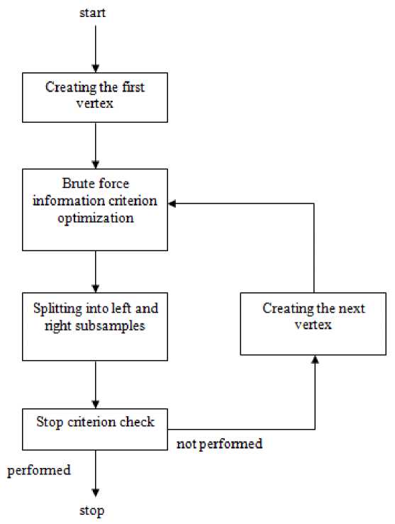
Fig. 1. Decision tree learning algorithm

Рис. 1. Схема алгоритма обучения дерева принятия решений

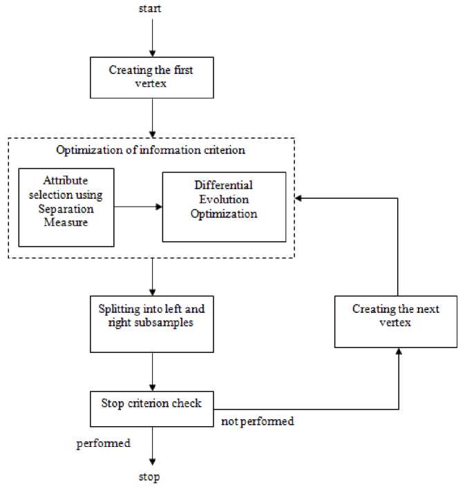
Fig. 2. Modified decision tree learning algorithm

Рис. 2. Модифицированный алгоритм обучения дерева решений

Probabilities are adapted on the basis of information about the successful or unsuccessful use of a mutation according to the formulas:

P i = P all + r i

⁽¹ - nP all ) scale

0.2 pall = , n scale = ^ r , i=1

success ²

r =------~- used

where n is the number of mutation types, used i is the number of applications of the i -type of mutation, success i is the number of successful applications of the i -type of mutation, i. e. when the fitness of the offspring exceeded the average fitness of the parent population.

In the differential evolution method, in addition to the mutation strategy there are two more important factors that need to be adjusted: F is a parameter that determines the strength of the mutation, i.e. the amplitude of disturbances introduced into the vector by external noise; Cr is a parameter indicating the probability of crossing. Adaptation of parameters is carried out according to the Success History Adaptation algorithm [11]:

oldp +

^F new = —2^ s - , where new F is the new value of the parameter F , and old F is the old one, respectively.

n si = ^ wi • (success _Fi)- , i=1

n

• s -    = ^ wi • success _ F i ,

i = 1

FitDifi

j = 1

where n is the number of the parameter F successful applications, i. e. when the fitness of the offspring exceeds the average fitness of the parental individuals; success_F is the value of the successfully applied parameter F ; FitDif is a change in the fitness value for each successful parameter.

The procedure is similar for the parameter Cr . Parameters are adapted on the basis of information on the success of their application.

Fig. 2 presents a modified diagram of the decision tree learning algorithm.

The solution of classification problems. 4 tasks usually applied to analyze the effectiveness of classification algorithms [12] were used to compare the well-known DT learning algorithms with the modified algorithm:

• 1)    Determining the type of soil from a satellite image.

• 2)    Determining the type of a car.

• 3)    Recognition of the type of an object by its segment.

• 4)    Recognition of the urban landscape.

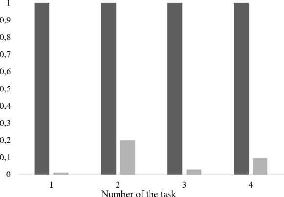
Comparison of algorithms is presented in the form of diagrams in fig. 3–6. It should be noted that the results averaged over 100 starts are presented for a modified learning algorithm with the differential evolution method, which is predetermined by the stochastic nature of the algorithm. Since the training time for standard and modi- fied algorithms is significantly different, it is not possible to display them on diagrams. Therefore, for clarity in the diagrams the training time of standard algorithms is taken as a unit, and the training time of a modified algorithm is represented as a fraction of the training time of a standard algorithm. The horizontal axis in the diagrams shows the numbers of tasks.

Fig. 3, 4 illustrate a significant reduction in the time spent on the learning process. The following are diagrams comparing the efficiency of the algorithms classification. Efficiency refers to the percentage of correctly classified test sample objects.

Fig. 5, 6 show that the results of the classification efficiency do not differ significantly.

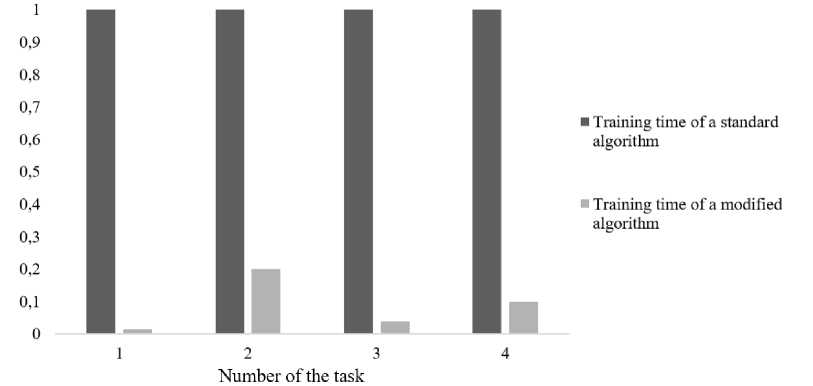
Fig. 3. Comparison of ID3 algorithms training time

Рис. 3. Сравнение времени обучения алгоритмов ID3

Time

■ Training time of a standard algorithm

■ Training time of a modified algorithm

Fig. 4. Comparison of CART algorithms training time

Рис. 4. Сравнение времени обучения алгоритмов CART

Efficiency

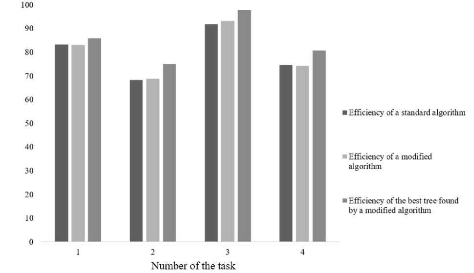
Fig. 5. Comparison of ID3 algorithms classification efficiency

Рис. 5. Сравнение эффективности классификации алгоритмов ID3

Efficiency

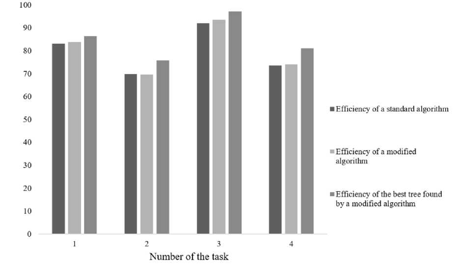
Fig. 6. Comparison of CART algorithms classification efficiency

Рис. 6. Сравнение эффективности классификации алгоритмов CART

Table 1

Experimental values of Student’s t-test (average values)

	ID3	CART
Task 1	0.263	0.77
Task 2	0.378	0.121
Task 3	1.017	0.963
Task 4	0.27	0.381

Table 2

Experimental values of Student’s t-test (best values)

	ID3	CART
Task 1	0.633	1.648
Task 2	2.635	1.506
Task 3	1.953	1.991
Task 4	2.389	3.097

Statistical analysis. Statistical analysis for a statistically reliable comparison of the efficiency of the standard and modified algorithms [13] was carried out in the present paper.

The hypothesis of the equality of mathematical expectations was put forward, an alternative hypothesis assumes inequality of mathematical expectations, the critical area is two-way. Cross-validation of each data set was performed, the algorithms were trained and tested several times on different parts of the samples in order to test the hypothesis. Student's t-test was used for comparison. According to Student’s distribution table, t cr = 2.101 was determined with a significance level of α = 0.05 [14; 15]. Tab. 1 shows the observed values of Student’s t-test for the considered taks. Each cell corresponds to t obs when comparing standard and modified algorithms.

All observed values of Student’s t-test from tab. 1 did not fall into the critical region, i. e. t _obs<  t _cr, therefore the hypothesis of mathematical expectations equality is accepted. Tab. 2 shows the observed values of Student’s t-test when comparing trees obtained by the standard algorithm with the best trees obtained by the modified algorithm.

In tab. 2 not all observed values of Student’s test exceed the critical indicator, therefore, not all the best trees found by the modified algorithm have statistically significant differences from the trees obtained by the standard algorithm. However, in tab. 2 bold indicates values that exceed the critical indicator; for tasks 2 and 4 the modified ID3 algorithm can find decision trees that cope with classification much better. Similarly, for task 4 the modified CART algorithm allows finding the best decision trees.

Conclusion. In accordance with the statistical analysis the following conclusion can be drawn: when using the proposed modification of the decision tree learning algorithm, the training process can be significantly accelerated without losing classification efficiency. In addition, it is worth noting that although on average the algorithms work the same way, modified algorithms sometimes allow finding decision trees that better cope with the task. In the future it is supposed to automate the process of forming decision trees by evolutionary algorithms in order to increase the efficiency of this method.