Diffractive optical power of a square diaphragm

The phenomenon of diffraction pulling or diffraction shift of image (focus) is at present being under the active investigation for as gaussian beams [1, 2] as spherical and cylindrical waves [3-8]. The approximate formulae for calculation of the diffraction focal shift for converging spherical light wave with different Fresnel numbers N have been proposed at the number of papers [4, 5, 6, 9]. Sufficiently accurate interpolation formula for the approximate calculation of the diffraction shift of image was found at [9], it is based on the concept of the diffractive optical power of a diaphragm.

We consider the focusing action of the diaphragm to be connected with the well-known peculiarities of Fresnel diffraction pattern. According to the theory of the wave diffraction at the semi-plane, the light field diffuses into the area of geometrical shade. Its intensity is increasing as it approaches the shade boundary, but at the boundary the intensity reaches only a quarter of the geometrical optics value. The light stripes are observed in the lighting area, the brightest stripe is the nearest to the boundary, and is 0. 86-JXz (% is the wavelength, z denotes the distance from the aperture plane) distant from it. The maximum intensity is 1.37 in the same units. Qualitatively, these peculiarities are retained also under the diffraction at an aperture of any form and dimension, i.e. the light stripes fringe the shade boundary only if the distance to the first light stripe does not exceed half the diameter of the aperture that is if the condition V%z < a is fulfilled. Any finer structure in the transversal intensity distribution cannot exist because the condition %z ~ a2 means that there can be only one Fresnel zone on the aperture. Hence, when the first light stripe of Fresnel diffraction pattern comes onto the geometrical optics axis of the diffracted wave, intensity distribution at transversal section of the beam is unstructured. The intensity at the beam axis appears greater than its geometrical optics values, and the intensity distribution at the beam transversal section at the distance z = a2/% becomes narrower than when the diffraction is not allowed for. This fact is interpreted as a focusing by the aperture and the definite optical power is attributed to the aperture. In its turn, the focusing apparently must result in the shift of the point source image. Thus the focusing and the diffraction shift of image are inherent in the apertures of arbitrary forms.

In the Fresnel parabolic approximation the modulus of the amplitude of the diffracted field | E ( 0 , z )| on the axis of a converging spherical incident light wave with the curvature radius R depends explicitly on Fresnel number N for the centre of the wave front curvature and on difference Z m = N_z - N ( N_z is Fresnel number for the current point z ) and implicitly on the aperture form that determines the domain of integration. A linear-hyperbolic interpolation with three parameters allows constructing the approximate analytical description of the diffraction shift. The difference of values Z m^act - Z m at two points and the difference of derivatives at one of them were reduced to zero.

Analytical expression for the z co-ordinate of the intensity maximum | E ( 0 , z )| has the form of a lens formula [9]:

1 z

R D ,

Ф

D

%          2 b

—---,         ^= a N - c + ^( N - c) + 4 bd

Where N = a ²/% R , a is the radius of the circular aperture (or the radius of the circumscribing circle in the case of the polygon aperture).

For the case of the aperture in the form of a rectilinear polygon with l side, the numerical values of the coefficients b, c and d are presented in the Table 1. Coefficients values demonstrate the convergence to the circular aperture ( l = ^ ) as the variable l is increasing.

The quantity Ф D can be considered as the optical power of the aperture due to the diffraction by origin. In addition to the factor %/ a² it contains the additional factor describing the dependence Ф D on N or on the wave front curvature 1 R . The precision of these equations proves to be as over the precision of the equations offered in [4 – 6] as ten times.

Table 1. Numerical values for coefficients

l	Z 0	b	c	d
^	1.000	12/ n 2= =1.2159	0.0357	1.2516
8	1.106	1.4793	0.0393	1.2452
6	1.192	1.6965	0.0410	1.2282
5	1.282	1.9152	0.0376	1.1940

In the case of the divergent incident wave, the question about the opportunity for the applicability of the diffractive optical power concept to the action of a diaphragm demands the additional analysis. The question is that the first light stripe of Fresnel diffraction pattern is not able to come onto the axis of the diffracted beam if ( R ( is sufficiently small quantity ( R <  0 ). In this specific case the physical basis of the concept is failed. This paper expands on the previous study [9, 10]. The possibility of the diffractive focusing of the divergent wave is considered. Special attention is given to the diffraction at the square diaphragm.

1.    A converging spherical incident light wave

Let us consider the modulus of the amplitude of the diffracted field | E ( 0 , z )| at the axis of a spherical incident wave with the curvature radius R . We center the origin of co-ordinates on the aperture. Analyzing Kirchhoff integral in the parabolic approximation, we will use the effective Fresnel numbers N and N_z defined through the radius a ₀ of the circumscribing circle:

N = aL , N = a ,                   (2)

z X-z X-R the difference

Z = N - N = 1I                      (3)

z

X V z R )

will be the main dimensionless variable.

With this specific notation the modulus of the field amplitude | E ( 0 , z )| can be written as

| E (0, z )| = (1 + N/Z) f (Z), f (Z) = Z JexP(inZ-r2)dr . (4)

Here r is the radius vector at the aperture plane, normalised on a ₀ . The co-ordinate z is measured from the centre of the aperture. The integral is evaluated over the surface of the aperture, using conventional normalisation the geometrical optics quantity is | e| = 1.

It can be seen the function E(0, z) explicitly depends on two parameters - N and Z, and implicitly -- on the aperture form, which defines the domain of integra- tion. Substantially, the function fZ) depends only on Z and the form of the aperture, and explicitly it does not depend on the radius of curvature R for the incident wave front. In this sense fZ) is universal, it equally describes the diffraction of plane, converging and diverging waves. The quantity R begins to influencefZ) only after the transition from Z to variable z by formulae (2) and (3). With variables N, Z the field amplitude depends on R only over the factor 1 + N/Z . The phenomenon of the diffraction shift for image is connected just with the factor 1 + N/ Z .

The variable Z is also convenient in the problem of calculation accuracy of the diffraction shift. Usually it is not the absolute value of the image position uncertainty 8z that is important but its ratio to the diffraction focal tolerance Az (length of the beam waist):

X zz a ²

z

N ^, z

8z8

— = N — = ^-8Z .

Azz

For a square aperture the function f ( Z ) in formula

• (4)    is expressed in terms of Fresnel integrals:

f (Z) = 2 [ c 2 (VZ)+s2 (TZ)],(6)

( _ X

C (^ Z ) = J cos I ^ t I d t , 0 V ^{2 )}

₍ n

S (V Z ) = J sin I — t I d t .

• 0 ^{V 2 )}

A plot of the function f ( Z ) is shown in Fig.1 (curve 1). In case of plane incident wave ( N= 0), the principal amplitude maximum is caused by maximum of the function f ( Z ) , which appears first as Z increases up to the value

Z = Z o = 1.4629.                                (7)

At this point f (Zo) = 1.801, f 2(Zo) = 3.244.                  (8)

A plot of the function f ( Z ) for the circular aperture is shown in Fig. 1 (curve 2). Here at the point Z = Z ₀ = 1, | E (0, z )| = 2, i. e. it is twice the value obtained from the geometrical optics, and the intensity is four times, and the transversal distribution has approximately half the width determined under the geometrical optics. Therefore, the diffraction focal effect of a square aperture is less (19%) than that of circular aperture.

The point of maximum intensity is given by the root

‘ of the equation E(0,z) = 0 from which the explicit form of the inverse function N (Zm) follows:

N ( Z m ) =

____________ Z m /² [ C (V Z m ) cos ( nZ m /2 ) + S (7 Z ; ) sin ( nZ m /2 ) ] ____________ c ² (vz ; ) + s ² (vz ; ) -c [ c (vz ; ) cos ( nZ m /2 ) + s (vz ; ) sin ( nZ m /2 ) ]

The function Z m ( N ) of interest is found by linear interpolation from calculated values of N ( Z _m ) .

Fig. 1. The function f ( Z ) for square and circular diaphragms (curve 1 and 2, respectively)

The behaviour of N ( Z _m ) in the limiting cases of small and large diffraction shifts is derived from equation (9) using the corresponding power expansions of trigonometric integrands:

N = iT^’ Z m <<  1,                    (10)

2 n Z

m

N = Y ( Z o -Z m ) , Z o -Z m <<  1,                (11)

where the coefficient

erture to be rather rough in fact. The form of pupil displays, in particular, in the difference of signs of the parameter c . We tried to apply Eq.(1) with numerical values of coefficients for circular aperture (from Tabl.1) to determine the focal shift in the case of a square aperture by substituting N by a N , where the coefficient a was found by the least square method. The optimal fitting yields the estimation error Z m equal to - 0.083 if N >2.68, and equal to 0.4 if N ^ 0 ( a =0.3758). In other words, diffraction shift with a square aperture and effective circular aperture are equivalent only with such accuracy. At the same time, approximation formula ensures much higher accuracy (~0.0015) with the proper choice (13) for coefficients.

2. A divergent spherical incident light wave

Now consider the divergent spherical wave diffraction at the square diaphragm. Ray tracing through the diaphragm is shown at Fig. 2. Here F is the point light source. The co-ordinate plane ( x , y ) is placed at the diaphragm plane. The observation plane is parallel to the diaphragm and is z distant. The typical plot of Fresnel intensity distribution I ( x ₀,0 ) at the observation plane ( x ₀, y ₀ ) is given at Fig. 2.

Y =

Z o [W Z 7 V c ² (7 Z 7 ) + s ² (T Z ? ) 2 [ c ² (VZ7) + s ² «_й) ]

^{- 1}

—0 = 2.1157 .

For the analytical description of the dependence Z _m on N, we propose the approximating formula, which is based on the asymptotic values (10), (11), and in which, instead of the trigonometric functions and Fresnel integrals, included in the ratio (9), the power series are used:

Fig. 2. Ray tracing through the diaphragm

^N = ^{- d}k ^Z m ^{+ C}k +Z k" . m

Three coefficients b k , c k , d k are defined according to the limiting values (10), (11):

b_k = 452 л ² = 2.2797; d k = y- b_k /Z 0 = 1.0500;

O k = d k Z 0 - b k /Z 0 =- 0.0230.                  (13)

Equation (12) allows one to get the analytical expression for the function Z _m ( N ) :

Z m =--------

N ^- C k ⁺

2 b k

V( N - C k ) ² + 4 b_kd_k

.

If we turn into the dimensional variables we will write (14) as (1).

The differences of the accurate and approximate values were numerically calculated from (9) and (14). The maximal error in equation (14) takes place for N =2.3 and is equal to 0.0015.

The attractive attempt to reduce the shift with a square aperture to the shift with an effective circular ap-

Let find the maximum value N (R<0) for the incident wave for which diffractive forming of the point image is possible in the sense, that the first light stripe of Fresnel diffraction pattern comes onto the axis of the diffracted beam. For the divergent wave the first light stripe maximum is x1 distant (Fig. 2) from the shade boundary. According to [11] the distance x1 is expressed by x1 = v1(1 + z/|R|)X zj2 , v1 = 1.21720 . (15)

At the plane ( x , z ) the first light stripe maximum describe the curve under the variation of z. The curve equation is

^{x ( z} ) =

-0 2 ^{( 1 +} z/|^R |^{) -} v ^^{( 1 +} z/|^R |) X z /² .

Under the condition |r| ^ ^ (the plane incident wave) the point z, in which the first light stripe comes onto the axis ( x = 0 ) , can be find from (16):

Z m = a 02 /1 v 2 , v 2 = 1.4816.                     (17)

According to (1) the exact value for z co-ordinate of the intensity maximum at the axis is equal to

z m = a 2 /( 1.4626 X ) . Thus the qualitative relations, based on Fresnel diffraction pattern characteristics, bring to the result differed from the exact calculation only by 1.3%. Formula (17) evaluate the diffractive back focal length for the diaphragm or 1 Ф D .

Let introduce the dimensionless variable Z = x] a , П = zJ\R and rewrite the equation (16) as

^(n) =1+n- v V n(1+n)/|n| == 71+n (л/1 + П - V 4 П/|k|)

The geometric loci for the first diffraction stripe maximum under the various N are given as curves at Fig. 3. Curves under the small N cross the optical axis and, therefore, the diffraction focusing is carried out for weakly divergent waves.

Fig. 3. The geometric locus for the first diffraction stripe maximum under the various N

The point n _m for the validity of the equation ^ ( n ) = 0 can be find from (18):

nm = V( v2/( k(- 1) .(19)

Hence, the focusing is actualised if

I k |< v2.(20)

Or in absolute values

|R\ > a2/(Xv2), -R > a2/(Xv2 ).(21)

The equality in the expression (20) and (21) evaluate the front diffractive focal length R of the diaphragm. This length coincides with the back diffractive focal length (17) up to a sign. That is, the well-known ratio for the perfect optical systems is satisfied in this instance.

If R <  a ₀ ² /( X v 1 ² ) than the diffractive optical power of the diaphragm is low to focus the real point image and it would be the virtual image ( n _m <  0 ) .

All of it becomes explicitly clear if to rewrite the equation (19) by the absolute value:

1 z m + 1 R = 1 / D , 1 f D =X W a 0 .        (22)

Then fulfil the analysis for the Fresnel diffraction integral. The intensity distributions along the z axis under x ₀ = 0, N <  0 and along the x ₀ axis under N< 0 (divergent waves) are of interest, that is the case of the one-dimensional problem is of interest. Let write the intensity at the point x ₀ ,0, z (Fig. 2) as

I ( Xo, z )= 2 (1 + N/ Z)

t ₂

j exp (jnt2/2) dt t1

t 1,2 =±Л^^- x 0 ^Nzf^ak 41 .

At Fig. 4 the plots show the intensity distributions at the optical axis in relation to z R at given N .

Fig. 4. The plots show the intensity distribution at the optical axis in relation to z R distance under various N

The units of measure for the intensity I are choose so that the quantity I is equal to 1.8014 under N= 0. The distinct maximum is observed in the curves for the absolute value of [ N ] satisfied the inequality: | k | < 1.4816. As [ N ] is growing the maximum location is displaced toward the bigger z values . This fact agrees with the “lens formula” (22). Maxima exist under | k | > 1.4816, but they are marked feebly. Transverse intensity distributions I ( x ₀, z ) in relation to x ₀ / a in the planes of the I ( 0 , z ) maxima are shown at Fig. 5. Value N is indicated as bracketed number above the curve. The corners mark the geometrical optics boundary of the shade for every curve at the Fig. 5. As the figure indicates the constriction of the lighted field has resulted from the diffraction at any case. The intensity maximum at the axis has the less height than it from Airy disk under N= 0 and the intensity do not decrease down to zero. The lighted field is enlarged and the intensity maximum height is decreased as far as | N | is growing. In the curve 3 (Fig. 5) the peak at the axis x ₀/ a = 0 is not delineated and the second peak is placed almost in the point x = a_k . This fact conforms to the analogy among the diffractive and the geometrical optics focusing: the value N =

–1.48 answers the light source position at the front focus of the diffractive lens when the half width of the beam would be equal to a k according to the geometrical optics.

In the curve 4 and 5 (Fig. 5) the maximum at the axis x 0 / a =0 is not observed, the focusing is absent in the case of N = –1.48.

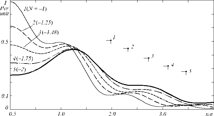
Fig. 5. Transverse intensity distributions I in relation to x ₀ a in the plane of I ( 0 , z ) maxima under various N

The root of the equation d E ( 0 , z )/d z = 0 gives the maximum intensity location Z _m at the axis. The explicit form (9) for the function N ( Z _m ) is correct for the negative N , too. The inverse interpolation function Z _m ( N ) coincides with (1).

The accuracy of approximate expression (1) is calculated with help of (9). The 100-fold magnified difference Z™ct - Z of the results of the direct determina-mm tion of the location of the intensity maximum and the calculation of Zm from approximating formula subject to N is illustrated by curve 1, figure 6. The error of the calculation of the image location from formula (1) does not exceed 0.15% of the diffraction depth of focus in the region -0.37 < N < ^ . In the region -1.48 < N < -0.37 the error grow and the accuracy of the approximate expression (1) decrease down to 2.86% for N = - 1.48.

In the case of negative N , the next more accurate interpolation formula for the maximum location has to be applied:

N =P/Zm +O-8Zm ,

Z =----------- , 2^е            =,                  (24)

m ,

N-о +д/( N-о) + 48P

where the coefficients p = 2.4330, о = - 0.2326 and 8 = 0.9783 are determined from the values in the point of interpolation:

N ₀ = 0, Z ₀ = 1.4626, dN/d Z|_z = _z =- 2.1157;

N 1 = - 1, Z 1 = 2.0172.

The curve 2 (Fig. 6) gives the difference (Zmact -Zm )x100 obtained with a help of (24) subject to N. The error of the calculation of the image location from formula (24) does not exceed 0.07% of the diffraction depth of focus in the region -1.015 < N < 0, then it increase as far as N decrease and it become equal to 1.0% under N = -1.4815.

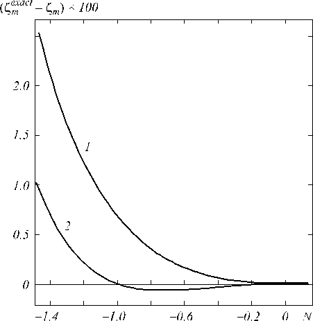
Fig. 6. The 100-fold magnified difference ( Z mac - Z _m ) of the results of the direct determination of the intensity maximum location and the calculation of Z _m from approximated formula (1) (curve 1) and formula (24) (curve 2)

3.    Conclusion

As a result of the consideration of diffractive shift of an image we have extended the concept of the optical power of a diaphragm over the case of square diaphragm and the negative Fresnel number. The high ap- proximation precision (0.07%) is the conclusive evidence for the correctness of our physical model for the focusing action of the diaphragms.