Динамика обратного рассеяния во время большой геомагнитной бури по данным Екатеринбургского радара: 17-22 марта 2015 г

In spite of multi-year experimental research, started with the aid of ionosondes in the 1920s, the study of ionospheric storms still remains one of the highest priorities in near-Earth space physics [Buonsanto, 1999; Mendillo, 2006; Goodman, 2005]. Its significance lies in the fact that the ionosphere has a great effect on telecommunication systems whose uninterrupted operation is necessary for humanity. The main difficulties in studying ionospheric storms are associated with the low spatial resolution and loss of ionospheric data during strong magnetic storms, as well as with the lack of detailed information about electric fields of magnetospheric origin (magnetospheric dynamo) and thermospheric processes affecting ionospheric storms. Some of these problems can be solved through a comprehensive analysis of data acquired with different instruments in a region of interest [Pokhotelov et al., 2008; Verhulst et al., 2014].

The review [Mendillo, 2006] shows that the loss and insufficient spatial resolution of data on the F2-layer peak electron density ( N m F2), obtained by ground-based ionosondes, can be compensated by total electron content (TEC) data. Recall that ionospheric storm intensity and phase are determined from disturbances in the critical frequency f _oF2 of this layer that makes the main contribution to TEC (see, e.g., [Bryunelli, Nam-galadze, 1988]). Spatio-temporal dynamics of electric fields emerging in the magnetosphere and transferred along geomagnetic field lines to ionospheric heights can be studied in detail in regions probed by radars [Ribeiro et al., 2011]. In Russia, such a comprehensive study can be carried out for the ionospheric region probed by the Yekaterinburg radar (YeKB radar) [Berngardt et al., 2015]. Unfortunately, due to the small number of GPS-receivers deployed in this region, TEC variations therein can be used only as an auxiliary instrument that provides information on possible N m F2 trends.

The geomagnetic storm which began on March 17, 2015 and was named the St. Patrick’s Day storm was the 13th intense geomagnetic storm of solar cycle 24 and the first during which the Dst index was lower than –200 nT [Kamide, Kusano, 2015]. Most published works on ionospheric effects of this storm rely on data from satellite navigation systems.

Analyzing GLONASS data, Tertyshnikov [2015] showed that during the first 8 hours of the main storm phase, TEC over Elbrus was higher, whereas during the remaining 4 hours and the next 4 days of the recovery phase it was lower than the mean values of this parameter in March 2015.

Jacobsen, Andalsvik [Jacobsen, Andalsvik, 2016] used for this study rate-of-TEC index (ROTI) values obtained from Global Navigation Satellite System (GNSS) data. Having compared the spatiotemporal dynamics of ROTI and equivalent ionospheric currents, calculated from IMAGE data, the authors found that the strongest GNSS signal disturbances over Norway were observed at the polar boundary of auroral electrojets, and attributed these disturbances to reconnections in the magnetotail.

Using ROTI maps, obtained with GPS in the Northern Hemisphere, Cherniak and Zakharenkova [Cherniak, Zakharenkova, 2015] show that the development and intensity of the high-latitude irregularities during this storm revealed a high correlation with auroral hemispheric power and auroral electrojet indices.

The authors of [Astafyeva et al., 2015] conducted a comprehensive analysis of satellite and groundbased data on TEC (including TEC in the top ionosphere), N e at 460 and 530 km, and the [O]/[N 2 ] ratio, determined from TIMED satellite data. The authors revealed significant increases in TEC of the top ionosphere in the dawn and dusk sectors and ascribed them to the increasing ratio [O]/[N₂]. Note that the information on N _mF2 variations during the storm given in [Astafyeva et al., 2015] does not reflect, in spite of the opinions of the authors, the global dynamics of this parameter because they analyze data only from ten widely spaced ionosondes located at latitudes from 57° S to 55° N.

The authors of [Liu et al. 2016] notice that TEC variations do not always correlate well with N m F2 variations during geomagnetic storms, and make a brief review of works which mention this fact. They 32

show that in the region with storm-enhanced density (SED), observed over North America at 16:00–24:00 UT on March 17, TEC values were higher, while N m F2 ones were lower than those at respective hours on March 16. Using COSMIC and GPS data (heights of ~800 and 20200 km respectively), the authors demonstrate that in this case TEC values were high due to the electron density above the F2-layer maximum. Yet the electron density in the lower ionosphere decreased due to changes in the composition of the neutral atmosphere. The results obtained in [Liu et al., 2016] suggest the need to further explore the relationship between TEC and N m F2 values in different geomagnetic conditions.

The first data on significant disturbances of the ionospheric radio channel during the St. Patrick’s Day storm was summarized in [Ponomarchuk et al., 2015] and discussed in more detail in [Polekh et al., 2016]. Using the oblique sounding data obtained along Norilsk–Irkutsk, Magadan– Irkutsk, and Khabarovsk–Irkutsk paths, the authors showed that the change in the magnetosphere structure during the initial and main phases of the geomagnetic storm (March 17) led to the occurrence of signals propagating outside the great-circle arc and the absence of radio signals propagating along the first two paths in the evening and night hours. The negative ionospheric disturbance developing during the recovery phase manifested itself over the same paths in a change of the mode structure in the daylight, evening, and night hours on March 18 and in the night hours on March 19, as well as in the 1.5–2-fold decrease in maximum observed frequencies along all the three paths. Later, disturbances of the ionospheric radio channel over subauroral paths partially passing through the field of view of the YeKB radar were examined in [Blagoveshchensky et al., 2016].

Having calculated the latitude of the main ionospheric trough (MIT) from empirical models, the authors of [Ponomarchuk et al., 2015] attributed the radio channel disturbances, observed on March 17, to the displacement of MIT to the latitude of Irkutsk (52.5° N, 104° E). The validity of this interpretation is confirmed by observations of airglow at the ISTP SB RAS Geophysical Observatory located in Tory (51° N, 104° E), i.e. 1.5° south of Irkutsk [Beletsky et al., 2015; Podlesny, Mikhalev, 2015]. According to these works, for five nighttime hours of the main storm phase, this observatory observed an intensification of the 630 nm atomic oxygen emission. The emitting area had the shape of a latitude oriented arc shifting equatorward as the Dst index decreased. Emissions possessing such properties are called stable auroral red (SAR) arcs. It has been experimentally proved that SAR arcs are conjugated with the region of interaction between hot ring-current and cold plasmaspheric particles, i.e. with the vicinity of plasmapause and thus with the MIT equatorial wall [Ievenko, Alekseev 2004; Spasojevic, Fuselier, 2009].

A significant shift of plasma boundaries of the magnetosphere toward low latitudes during the St. Patrick’s Day storms was experimentally found in [Le et al., 2016]. According to that work, during the main storm phase, zone-1 field-aligned currents and the auroral oval shifted in the daytime magnetosphere to geomagnetic latitude of ~ 60°. Figures 3 and 5 of that article allow us to determine the latitude of the auroral oval and field-aligned currents of zones 1 and 2 in the YeKB-radar field of view for three time intervals. We take this opportunity in Section 5.

The results received in [Ponomarchuk et al., 2015; Beletsky et al., 2015; Podlesny, Mikhalev, 2015] confirm the well-known tendency for auroral phenomena to shift to middle latitudes as geomagnetic activity increases. However, these papers do not provide detailed information on spatio-temporal dynamics of this process. This information is required to examine relationships between ionospheric and magnetospheric–heliospheric disturbances during magnetic storms. The aim of our work is to gain such information through a comprehensive analysis of ionospheric and geomagnetic disturbances observed within the YeKB-radar field of view during the storm.

In the study, we will supplement YeKB-radar data with data from riometrtic, ionospheric, and magnetic stations located in its field of view and in its vicinity. Section 2 provides information about the region of interest and sources of the data under study. Section 3 briefly characterizes the magnetic storm and its heliospheric sources. In Sections 4 and 5, we compare changes in characteristics of backscattered signals with changes in ionospheric parameters, determined from ionosonde data and TEC maps, as well as with riometric and geomagnetic disturbances, observed during the storm within the YeKB-radar field of view. The main results of the study are presented in Section 6.

2.    DATA

The study relies on data from the coherent decameter YeKB radar (56° N, 58° E), acquired on March 16– 22 and for comparison on March 13–14, 2015 (magnetically quiet days). Technical characteristics of the radar are given on the website ; the basic principles of its operation and data processing techniques, in articles [Berngardt et al., 2015; Mager et al., 2015]. On the days considered, the YeKB radar operated at ~ 11 MHz in the normal mode along 0–15 beams providing spatial resolution of 45 km and temporal resolution of 1–2 minutes. Similar to Super Dual Auroral Radar Network (SuperDARN) radars, the YeKB radar measures the autocorrelation function of backscattered signals. Then, the standard method is used to determine characteristics of received signals [Ponomarenko, Waters, 2006]. In our work, we utilize the following:

P l – the signal-to-noise ratio,

V D – the Doppler velocity along the radar beam (positive toward the radar and negative away from it)

w – the spectral signal width,

R – the range.

For brevity, below we designate the power as P l , backscattered signals as BS signals, scattering ionospheric irregularities as FAEDIs (field-aligned electron density irregularities), and use the subscript i and g to denote signals scattered by FAEDIs and ground irregularities respectively [Blanchard et al., 2009]. Other rare notations will be introduced in the respective sections of the article.

To separate BS i signals, we adopt the criterion I V D I > 50 m/s, w >  30 m/s [Oinats et al., 2015]. Corrected geomagnetic coordinates of the i and g backscatteres (latitude ф' and longitude X' ) are determined by the standard model AACGM, used for SuperDARN data [Baker, Wing, 1989].

Paths of 0–15 radar beams, numbers of which increase from west to east, are shown in Figure 1. Circles mark positions of 7 of 11 ground-based stations whose data are used in this work. Names, geographical and corrected geomagnetic coordinates of the stations and their IAGA/URSI codes are listed in Table 1. In the corrected geomagnetic coordinate system, the radar field of view covers 55–80° latitudes and 131.5–184.5° longitudes. This corresponds to the 3.5-hour sector of magnetic local time (MLT).

The analysis rests on the solar wind and IMF (interplanetary magnetic field) data from the ACE satellite [ftp: // ]; TEC values and magnetic measurements from AARI observatories [http: //]; INTERMAGNET data [http: // php]; riometer absorption plots []; ionograms taken from []; geomagnetic indices, magnetic and ionospheric data from ISTP SB RAS observatories.

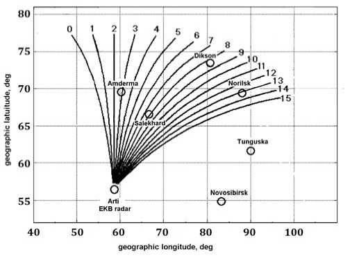
Figure 1. Paths of 0–15 YeKB-radar beams and the position of ground-based stations in the geographic coordinate system

Table 1. Coordinates of magnetic (m), ionospheric (i), and riometric (r) stations

№	station	IAGA/URSI code	coordinates
			geographical		corrected geomagnetic
			latitude	longitude	latitude	longitude
1	Diksonm,i,r	DIK/DI373	73.5	80.7	69.4	156.3
2	Amdermam,r	AMD	69.6	60.2	65.9	136.5
3	Norilskm,i	NOK/NO369	69.4	88.1	65.5	162.5
4	Salekhardi	SD266	66.5	66.5	62.9	141.4
5	Tunguskai	TZ362	61.6	90.0	57.9	163.9
6	Artiem	ARS	56.4	58.57	53.0	132.1
7	Novosibirskm	NVS	54.8	83.2	51.2	156.7
8	Pevekm	PBK	70.1	170.9	65.8	232.1
9	Tiksim,r	TIK	71.6	128.8	66.5	198.6
10	Yakutskm,i	YAK/YA462	62.0	129.6	56.8	202.1
11	Abiskom	ABK	68.4	18.8	65.6	100.8

Corrected geomagnetic coordinates of ground-based stations (latitude ϕ′ and longitude λ′) are calculated using the software available at [ ]. Magnetic data from AARI are presented on the above website by components Bn, Be, and Bz directed to the north, east, and down vertically respectively.

3.    HELIOSPHERIC AND GEOMAGNETIC DISTURBANCES

According to Dst values, the St. Patrick’s Day magnetic storm began after 04:00 UT on March 17, peaked by the end of the day, and ended after 14:00 UT on March 25. The storm onset was preceded by 8 days of low and moderate geomagnetic activity. From March 9 to 15, the A p and Dst indices changed within 4–9 and –14–18 nT. Geomagnetic activity went up on March 16. The indices rose up to A p = 12 and Dst = 2–29 nT.

More detailed information on the ring current dynamics is provided by the plot of SYM-H index variation, which is given with the plots of Dst , K p , and AE indices in Figure 2, a . By the SYM-H variation, intervals 04:45–06:22 and 06:23–23:06 UT on March 17 correspond to the initial and main phases of the storm. The moment of sudden storm commencement (SSC) and the beginning of the main phase are marked with vertical dashed lines labelled SSC and M respectively. The main phase consisted of two steps [Kamide et al., 1998]. The line labeled M₀ indicates the first minimum of the SYM-H index at 09:37 UT; the line designated by M₁, the beginning of the second decrease in SYM-H at 12:07 UT (the beginning of the second step).

We have noted above that the Dst index became positive in the second half of March 25. However, a relatively fast and stable growth of Dst and SYM-H was observed only from 23:06 UT on March 17 to 17:57 UT on March 18. For the first 70 minutes, the average rate of change in SYM-H (Δ SYM-H /ΔUT≈53 nT/hr) was 7 times higher than in the next 17.5 hours (Δ SYM-H /ΔUT≈7.6 nT/hr). This gives grounds to define the intervals 23:06–00:15 UT on March 17–18 and 00:16–17:57 UT on March 18 as the early recovery phase and a part of the late one [Dasso et al, 2002.]. In Figure 2, beginnings of these intervals are marked with lines R and R 1 . The line R 2 indicates the end of the steady growth of SYM-H . To determine background values of ionospheric parameters, we have chosen March 13 and 14 – the days of relatively low geomagnetic activity.

According to information posted on [], the 17–25 March 2015 geomagnetic storm developed under the impact of high-speed streams from four coronal holes and interplanetary coronal mass ejection. The source of geomagnetic disturbances during the first step of the main phase was a corotating interaction region (CIR); at the second, a combination of CIR and interplanetary coronal mass ejection (ICME).

Variations of four external parameters that have the major impact on near-Earth space are shown in Figure 3. These are the B z and B y IMF components (IMF B z and IMF B y ), the velocity ( V sw ), and the ram 36

pressure ( P sw ) of the solar wind. Plots are built from ACE data (coordinates x , y , z GSE ~ 220, –8, –23 R E ) for 00:00–24:00 UT on March 16–22. At that time, the satellite was at a distance (23÷27) R E from the Sun–Earth line and, consequently, gave adequate information on parameters of the interplanetary medium at the boundary of the magnetosphere [King, 1986; Ericsson et al., 2000]. The plots are drawn taking into account the transfer time of each heliospheric plasma fragment from the satellite to the magnetosphere, ΔUT=( x GSE – R mag )/ V sw . Here, R mag is the magnetopause standoff distance under the pressure balance. Vertical dotted lines are the same as in Figure 2. The bottom panel of Figure 3 plots the magnetospheric convection field E c calculated from V sw , P sw , IMF B y and B z (we use formulas given in [Burke et al., 2007]).

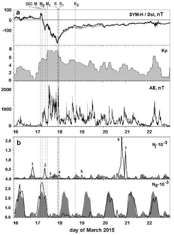
Figure 2. For March 16–22, from top to bottom are variations in SYM-H / Dst (black/gray line), K p and AE indices of geomagnetic activity ( a ) and in the number of BS_i and BS_g signals received by the YeKB radar per an hour on March 13–14 (gray shading) and 16–22 (black lines) ( b )

As inferred from ACE data, about 05:00 UT on March 17, the solar wind velocity near Earth increased abruptly from 400 to 500 km/s and remained high ( V sw ~ 600 ± 50 km/s) until the end of March 25. Comparing Figures 2 and 3, we can see that just after SSC there is a slight, short-term (about 10 min) increase in the AE index of auroral activity to 270 nT. The beginning of the main phase (point M) corresponds to a decrease in P _sw, the transition from positive to negative B_z , and an increase in E _c up to ~ 1.2 mV/m.

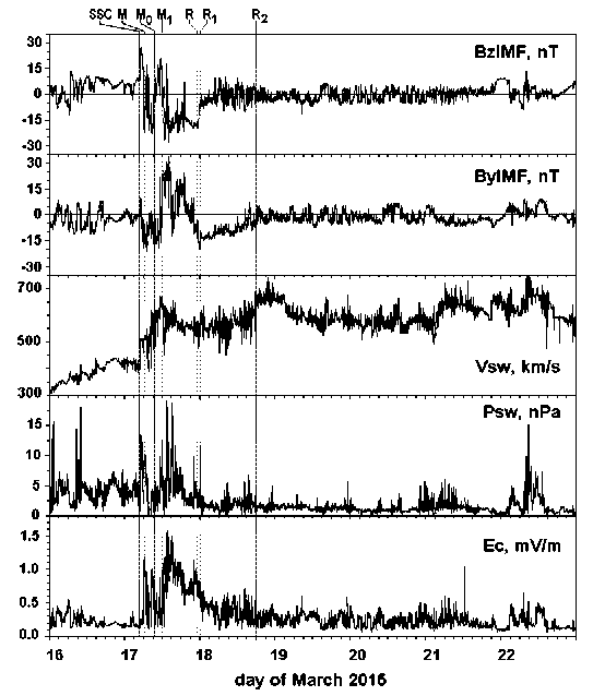
Figure 3. Variations in IMF B z and B y , velocity and ram pressure of the solar wind plotted from ACE data. The bottom panel shows variations in the magnetospheric convection field ( E c ) calculated from these data

During the first step of the main storm phase, there was a bay-like increase in AE to ~1000 nT in the interval M–M 0 (with B z varying from –22 to 17 nT) and its reduction to ~ 200 nT within M 0 –M 1 (IMF B z varied from –4 to 20 nT). Throughout the first step, IMF B y <0. The ram pressure of the solar wind monotonically decreases from 10 to 2 nPa (lower than that before the storm commencement), and then increases to the average P sw ~ 8 nPa at 10:30–11:30 UT.

During the second step of the main phase, IMF B z is largely negative, B y is positive; the convection field is strengthened to the maximum values E c ~ 0.7–1.5 mV/m for this storm. At 12:56–15:11 UT, we can see the highest AE peak of ~ 2300 nT corresponding in time to two most significant increases in P sw up to ~ 18 nPa (12:30–15:00 UT in Figure 3), the first of which was accompanied by a short-term northward rotation of IMF B z . The main peak is followed by multiple increases in AE up to 1500–1800 nT, which have no explicit relation to changes in heliospheric parameters. This is typical of the magnetosphere that is unstable during magnetic storms. In such cases, sporadic increases in auroral activity can be caused even by the slightest changes of conditions at the boundary of the magnetosphere [Bargatze et al., 1985; Sharma et al., 2005].

The early recovery phase of the storm (the R–R 1 interval) started with a sharp decrease in P sw from 4 to 2 nPa and attenuation of E c from 0.9 to 0.5 mV/m. In the early recovery phase, there was a bay-like increase in AE to 2145 nT at 23:45 UT. This AE maximum corresponds in time to the P sw jump from 2 to 11 nPa.

By the end of the early recovery phase, IMF B z reached –5 nT, P sw , ~ 1.5 nPa, E c , ~ 0.5 mV/m. At the late recovery phase, IMF B z ranged from –10 to 5 nT, P sw = 0.5–2 nPa, the average value of E c decreased to ~ 0.25 mV/m. At 01:00–07: 30 UT on March 18, AE ≤400 nT. Then, auroral activity went up. At 08:32, 11:19, and 14:57 UT there are peaks of AE = 1286, 870, and 1647 nT respectively.

To facilitate the comparison with information given below, basic information on geomagnetic disturbances of March 17–18 and their possible extramagnetospheric triggers are given in Table 2.

4.    DYNAMICS OF SIGNALS BACKSCATTERED BY GROUND

Let us consider characteristics of BS g signals observed on March 17–22 and on days of low and moderate geomagnetic activity, March 13, 14, 16. Start with daily distributions of N _g (the number of BS_g signals received by the YeKB radar per hour, see Figure 2, b ). It is evident that the day before the storm, March 16, N g variations were similar to those observed during magnetically quiet days. The plot of R g (UT), given in Figure 4, is also similar to those drawn for March 13–14 (not shown in the figure). It illustrates the typical diurnal variation in the range of BS g signals detected by midlatitude radars. They are characterized by gradual decrease in the range from maximum nighttime R g = 2500–3000 km to minimum daytime R g = 800–1500 km and by an increase in R g in the evening [Bland et al, 2014.; Mager et al., 2015]. This diurnal variation in R g is due to diurnal variations in N m F2 and the F2-layer peak height ( h _mF2). The values of N _g are maximum in the daytime (04–10 UT, N _g>2500) and minimum in the evening (13–16 UT, N g <300). The increase in N g occurs with an increase in the maximum power P lg .

Differences between the BS g signals received on March 17–18 from the signals observed at the same hours on March 13–14 manifest themselves in the following.

• (i)    Increasing number of BS g signals within 05:00–09:00 UT on March 17 by ~1000 relative to background N g .

• (ii)    Wavelike decreases in minimum R g within 04:45–12:00 UT on March 17.

• (iii)    A sharp decrease in N _g after 18:00 UT on March 17.

Comparing the plot of N g (UT) with plots of f o F2 (UT), shown in Figure 5, we can see that the peak of N g , noted in (i), occurs an hour before the peak of f o F2, observed only at the DI373 station between 06:00–08:10 UT (maximum f o F2 = 8.46 MHz at 07:25 UT). On the plot of R g (UT) (Figure 4) to this N g peak corresponds the band of BS g signals coming from 2100–2300 km (0–8 beams, 74–77° latitudes). Considering data from Table 2, we believe that the compression of the magnetosphere in the initial phase and within the first two hours of the main phase along with the reconnection on the daytime magnetopause [Le et al., 2016] caused an increase in the critical frequency of the F2 layer at 74–77° N in the sector 08:00–13:00 LT. This showed up in the growth of f o F2 over the station Dikson (73.5° N, close to the 8th beam) and in an increase in the number of BS g signals received by 0–8 beams. In Figure 6, the TEC plots drawn from 15-min values are compared with the plots of N m F2, calculated from 15-min values of f o F2. It is apparent that at the station Dikson to the N m F2 peak corresponds the TEC peak. At stations lo-39

cated further south, only the TEC peak is seen; its maximum shifted from NO369 to SD266 and TZ362 for 75 minutes. It is possible that the breakdown of correlation between TEC variations and N m F2 in this case is explained, as in [Liu et al., 2016], by an increase in the electron content of the top ionosphere that has not extended to heights probed by ionosondes.

The feature of BS g signals specified in (ii) manifested itself in the fact that between 04:45–12:00 UT the lower boundary of their ranges decreased to 700 km at ~ 05:00 UT, to 600 km at ~ 07:20 UT, to 700 km at 08:40 UT, and to 400 km at 10:30–11:30 UT. Comparing R g variations with data from Table 2 on SYM-H variations and AE peaks, we can see that the first decrease in the minimum range occurred after SSC; the second and third, after the bay-like increases in auroral activity. The fourth, the last decrease in R g occurred with an increase in SYM-H index (the beginning of the interval M 0 –M 1 , Table 2), which developed after the transition to IMF B_z >0 and an increase in the solar wind ram pressure (Section 3). Figure 5 shows that at that time on ionograms from the NO369 station ionospheric reflections disappeared, and then they appeared on ionograms with f o F2 values reduced to ~60–80% of the quiet level at 10:30–12:15 UT. The SD266 and TZ362 stations observed fluctuations of f o F2 with 30–120 min periods and ~0.5–2 MHz range, which after 13:00 and 12:30 UT were followed by the absence of reflections from the F2 region.

Let us discuss the decrease in the number of BS g signals noted in (iii). Figure 2, b indicates that at 12:00–17:00 UT N g values were close; and at 15:00 UT, they were even 2.5 times higher than at the same hours on March 13–14.

Between 18:00–14:00 UT on March 17–18, the number of BS i signals decreased to ~2–25 %; at 18:00–24:00 UT on March 18, to ~0.3–11% of background values.

Figure 5 shows that the NO369, SD266, and TZ362 stations from 13:00 to 23:00 UT and the DI373 station from 12:00 to 16:40 UT on March 17 observed sporadic E layers with f o E s close to the background f _oF2 or exceeding them. This indirectly indicates that a possible reason for the absence of reflections from the F2 layer, and in several sounding sessions, from the entire ionosphere, as well as for the significant decrease in N g was not the electron density decrease in the F2 region but its increase in E and D regions of the ionosphere. The comparison of TEC plots with N m F2 ones (Figure 6) suggests that there are no reflections from the F2 layer even when TEC values over the stations exceed background ones. This favors the assumption we made. It is not excluded, however, that in this case, large TEC values are associated with increasing electron density in the top (above the F2-layer maximum) ionosphere and do not correlate with N m F2 over the stations. The effect of the absence of reflections at high TEC values was most pronounced on March 17 at 14:00–17:00 UT. Over this UT period, plots of all the stations exhibit a TEC peak, the height of which above the background level is maximum at the TZ362 station (~ 8 TECU at 15:00 UT) and minimum at the DI373 station (~1.5 TECU at 15:30 UT).

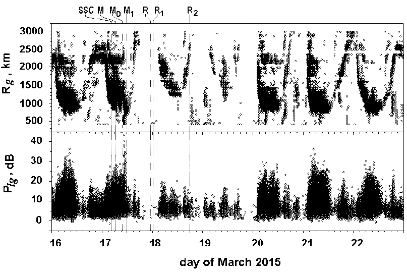
Figure 4. Variations in R _g and P _lg ground backscattered signals on March 16–22, 2015.

Figure 5. Variations in the critical frequency of the F2 layer ( f o F2) and the limited frequency of the E s layer ( f o E s ) over three stations located within the YeKB-radar field of view, and over the TZ362 station, situated 6.3° south of the radar, for March 17–19, 2015. Variations in the current values of f o F2 are shown by thick lines and squares, the background ones, by thin lines; f o Es, by triangles

Table 2. Geomagnetic disturbances on March 17–18 and their possible triggers. The UT/UTmax column contains time of observation of AE peak/maximum. The values of AE at the maximum are given in the column “maximum”

Interval	UT	storm phase	AE peaks
			UT/UTmax	maximum, nT	possible trigger
SSC-M	04:45– 06:22, March 17	initial phase	04:45–04:54/ 04:47	269	Δ P sw >0
M–M 0	06:23– 09:37, March 17	main phase, first step	06:09–07:09/ 06:38 07:12–10:36/ 08:52	772 1016	Δ P sw <0, ΔIMF B z >0 E c increase Δ P sw >0, Δ B z <0 E c increase
M 0 –M 1	09:38– 12:06	main phase, SYM-H increase	no		transition to IMF Bz >0 E c decrease
M 1 –R	12:07– 23:05, March 17	main phase, second step	12:56– 15:14/13:58 16:14–21:53	2298 many maxima at 1200–1900	Δ P sw >0, ΔIMF B z <0 E c increase undetermined
R–R 1	23:06– 00:15, March 17– 18	early recovery phase	23:14–24:00/ 23:17 23:42	1731 2145	Δ P sw <0, ΔIMF B z >0 Δ P sw >0, ΔIMF B z >0, ΔIMF B y >0
R 1 –R 2	23:07– 17:57 March 17– 18	a part of the late recovery phase	07:41–12:58 08:32 14:01–17:38 14:57	1286 1647	undetermined Δ P sw >0, ΔIMF B z <0

On March 18 at 00:00 UT, the situation changed rapidly. TEC values over NO369, SD266, and TZ362 reduced to ~ 35–45% of the background level. The stations occasionally observed reflections from the F2 layer with low NmF2 being ~ 20–30 % of background values. The moment 00:00 UT corresponds to 06:00 MLT in Norilsk and Tunguska, to 05:00 MLT in Salekhard. At YA462, located 3 hours further east and close to the latitude of TZ362, the transition to low TEC occurred 3 hours earlier – at 21:00 UT (~ 06:00 MLT) on March 17. Plots from YA462 are shown on the bottom panel of Figure 6. All this points to the fact that at the end of the main phase of the geomagnetic storm in the vicinity of the dawn meridian there appeared a sharp western boundary of the negative ionospheric disturbance related to the change in the composition of the neutral atmosphere. Indeed, the area of [O]/[N2] <0.5 with sharp boundaries is seen on the map of latitude-longitude distribution of this parameter, which is drawn for March 18, 2015 on the website []. On March 18, the western, eastern, and equatorial boundaries of low values of [O]/[N2] were at 80° E, 150° E, and 25° N respectively. Figure 8, c from [Astafyeva et al., 2015] illustrates that at 03:00–06:00 UT on March 17 at 55–80° N, 50–100° E (in the YeKB-radar field of view) [O]/[N2] was ~ 0.5, and at the same time on March 18, it fell to ~0.1.

5.    DYNAMICS OF SIGNALS BACKSCATTERED IN THE IONOSPHERE

]In Figure 2, b , numbers 1–7 denote peaks with N i being 3–40 times greater than at the respective hours on March 13–14. In Figure 7, a , to the first and 3–7 peaks correspond isolated discrete R i structures formed by clusters of points; to peak 2, the end of the series of discrete structures of diminishing range. Ribeiro et al. [Ribeiro et al., 2011] show that such clusters of points gather in scattering by FAEDIs, and their Doppler velocities can be used to determine the direction of the electric field component perpendicular to the radar line of sight (see also [Davies et al., 1999; Milan, Lester, 2001; Makarevich et al., 2009] and references therein).

Figure 6. TEC and N m F2 variations over the five ionospheric stations. The stations’ names are given on the panels. Current and background TEC values are depicted by thick and dotted lines respectively; N m F2, by the thin line with squares and thin line

Given the importance of this problem, we consider the dynamics of discrete BS i structures and compare it with the development of geomagnetic disturbances.

The structure designated by number 1 in Figures 2, b , and 7, a , is shown in Figure 8, a . In this case, the scattering points form a narrow horizontal strip ( ϕ′ = 66–69°) being consistently observed for three hours at low auroral activity ( AE ~ 30 nT). A similar, but wider structure ( ϕ′ = 62–68°), shown in Figure 8, b , was recorded on March 14 at AE ~ 180 nT in the recovery phase of the weak, ~ 200 nT geomagnetic disturbance, observed only at Dikson.

The widest horizontal structure, denoted by 6, is illustrated in Figure 8, c, together with structure 7. Structure 6 evolved at ϕ′ = 60–70^o during relatively high auroral activity ( AE ~ 80–600 nT). It appeared during the growth phase and disappeared at the end of the recovery phase of the ~600 nT bay-like negative geomagnetic disturbance, observed in Norilsk and Amderma. The BS i signals emerged in the growth phase of the bay-like disturbance, disappeared in its maximum, and re-emerged in the recovery phase. Judging by the signs ⊕ H <0, ⊕ Z > 0, at the minimum of the bay at 19:00–20:00 UT, accompanied by the peak of riometer absorption, the center of the western electrojet was south of NOK and AMD, and BS i signals were absent.

day of March 2015

Figure 7. Variations in R i ( a ), P li , and V Di of signals backscattered in the ionosphere; H component at the three auroral stations ( b )

At Dikson at that time there were three bays with ⊕ H ~ 200 nT (Figure 7, b ), which coincided with the AE peaks. The maps drawn for the discrete structure show that the radar field of view moved from the region of meridional flows directed toward the radar into the region of zonal flows directed away from the radar. The maps indicate that the equatorial boundary of FAEDIs shifted to ϕ′ i ~ 60° during the event. Over the observation period, the radar field of view shifted from the 21:00–00:30 MLT sector to the 01:00–04:30 MLT one.

The maps presented in Figure 8, a , b and for March 20 in Figure 8, c show that FAEDIs with V Di > 0 (<0) were seen in pre-midnight and midnight hours mainly in the western (eastern) part of the radar field of view. The presence of longitudinally spaced regions with different signs of V Di at ϕ′ = 60–70° indicates that during their observation in the radar field of view there were two regions with enhanced magnetospheric convection. These are (1) the western region in which E _c, perpendicular to radar beams, is north-westward (from dawn to dusk) and V Di > 0, and (2) the eastern region with south-eastward E c and V Di <0. The first region corresponds to antisolar ionospheric plasma flows; the second, to the western electrojet. The fact that these two regions were observed near midnight as well as the longitudinal separation of FAEDIs with different drift directions allow us to assume that these phenomena occurred in the vicinity of the Harang discontinuity.

Unlike them, horizontal structures 5 and 7, shown in Figure 8 c , d , were observed in the morning between 04:00–09:30 MLT after multiple amplifications of the western electrojet, which occurred with an increase in the absorption at AMD. In both the cases, in the region probed by the radar, the field of the western electrojet was maximum at AMD, over which, after the absorption reduced to 1 dB, scattering FAEDIs with V _Di<0 were detected. The average Doppler velocity of ~ –90 m/s was 1.5–2.5 times lower than that in the horizontal structures observed in the near-midnight hours.

The discrete R i structures, detected during the main, early and late recovery phases, significantly differ in the spatio-temporal dynamics from horizontal R _i structures. They are illustrated in Figure 9, b with temporal resolution that is higher than in Figure 7, a . Figures 7, a and 9, b show that at 06:20–11:30 UT on March 17 BS i signals formed an almost continuous series of discrete structures of diminishing range. The series is designated by number 2 in Figures 2, b , and 7, a . At the beginning of the series, R i ~ 2600 km, V Di are predominantly negative; at the end of it, R _i ~ 700 km, V _Di is largely positive.

The first element of the series appeared at the beginning of the first step of the main phase against the increase, and the last one, an hour before the beginning of the second step of the main phase against the decrease in PCN / PCS and AE . The increase/decrease in PCN / PCS indices indicates a strengthen-ing/weakening of the interplanetary electric field and hence of the magnetospheric convection, manifested itself in the increase/decrease in the AE index [Troshichev et al., 2006].

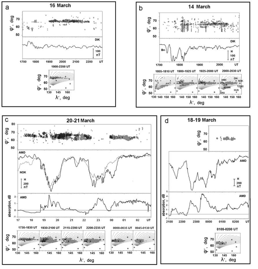
Figure 8. Variations in the corrected geomagnetic latitude ϕ′ of ionospheric backscatter, in the H component at one of the stations located within the radar field of view, and maps of scattering points in the corrected geomagnetic coordinate system for 17:00–23:00 UT on March 16 ( a ), 17:00–21:00 on March 14 UT ( b ), 17:00–03:00 on March 20–21 UT ( c ), and 00:00–03:00 on March 19 ( d ). H variations at NOK (gray line) and AMD (black line) plotted for March 20–21. Riometer absorption at AMD is plotted for the same days and for March 18–19. In Figures 8–10, ϕ′ i (UT) plots and FAEDIs maps are drawn for signals with P _li > 5 dB (the lower quartile of P _l values for March 13–14); gray symbols mark signals with V Di <0; black ones, with V Di > 0. Above the maps are their UT intervals

ит

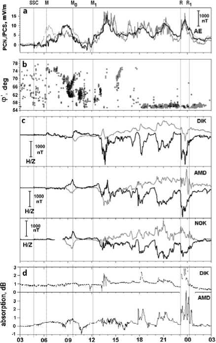
Figure 9. Variations in PCN / PCS / AE indices (black/dashed/gray lines) ( a ), in the corrected geomagnetic latitude of FAEDIs ( b ), in the H / Z geomagnetic field components (black/gray lines) recorded in the field of view of the YeKB radar ( c ), in the riometer absorption at DIK and AMD ( d )

The spatio-temporal dynamics of FAEDIs, which form the series, is depicted in Figure 10 (maps 1–7). The first element of the series is formed by signals with V Di ~ –600 m/c, observed along 0–4 beams and ϕ′ i ~ 73.6–75.4° at 10:50–12:20 MLT (map 1). The next element with the same characteristics is shown on map 2. The third element, observed at 08:00–09:00 UT along 0–7 beams, 5° further south than the first two, was also formed by FAEDIs with V _Di<0. Figure 5 shows that the appearance of this element is followed by the first significant decrease in the F2-layer critical frequency by ~ 3 MHz over Dikson and Norilsk. Map 3 illustrates its part that do not overlap in time with the next discrete structure formed by signals with V Di >0. When observing the third element, PCN / PCS , and AE indices are maximum.

We think that during the events presented on maps 1–3, the YeKB radar recorded FAEDIs located in the throat of enhanced magnetospheric convection. Such events observed by the SuperDARN radar near the noon meridian are described, for one, in [Fiori et al, 2009], by the YeKB radar, in [Berngardt et al., 2015]. Judging from variations in the H component (Figure 7, b ), which are negative in Abisko and positive in Pevek, at 06:00–09:00 UT on March 17 the YeKB radar did explore the ionospheric region situated between the dawn and dusk convection cells.

Maps 4 and 5 show two regions with FAEDIs – the western with V Di <0 (0–8 and 0–5 beams at the beginning and end of the event respectively) and the eastern with V Di > 0 (8–15 beams). They were seen in the afternoon sector when polar ( PCN ) and auroral ( AE ) magnetic activity went down, and were accompanied by the transition of the YeKB-radar field of view from the throat into the sector of the dusk cells of magnetospheric convection. This is evidenced by the positive bay in the H component, which is clearly visible on all plots of Figure 9, c .

Comparing geomagnetic field variations at the stations, we see that until M 0 the positive bay in H was observed at NOK and AMD. The electrojet center was located to the south of these stations (Δ Z <0). After M 0 , which, according to Table 2, corresponds to the transition to IMF B z > 0 and magnetospheric convection weakening, stations in Norilsk and Amderma recorded a decrease and on Dikson an increase in the eastward electrojet field whose center shifted poleward and stayed to the south of Dikson until the end of the bay-like disturbance. The maps show separation of the eastern region into two zones, spaced apart by Δϕ′ ∼ 3° and 5° (maps 4 and 5 respectively). Until M₀ in the zone located further south of NOK and AMD, the mean V Di was ~ 420 m/s, and after the moment it decreased to 390 m/s. However, in the northern zone, the Doppler velocity of BS i signals after M 0 rose from 370 to 470 m/s. We believe that the dynamics of FAEDIs we revealed indicates the presence of two zones of northward enhanced electric field, typical for the eastward electrojet, at 08:45–10:00 UT. After the change of the IMF B z sign from negative to positive, the meridional component E c decreased in the southern zone, but increased in the northern one. This caused the geomagnetic disturbances to weaken at NOK and AMD and strengthen at DIK.

Map 6, drawn for the interval 10:15–10:45 UT, displays only the region of FAEDIs with low positive Doppler velocities VDi ~ 70 m/s. Its respective PCN/PCS, and AE indices were low; the magnetic stations detect the end of the recovery phase of the positive bay-like H-component disturbance. The southern boundary of FAEDIs is located at the lowest latitude for this series – ϕ′i ~ 60°. When observing this structure, the critical frequency of the F2 layer at SD266 and TZ362 decreased by ~ 2 MHz, the ri- ometric absorption at AMD, to ~ –1 dB (Figure 9, d).

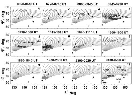
Figure 10. Maps of ionospheric scatters in the corrected geomagnetic coordinate system for the main, early and late recovery phases of the St. Patrick’s Day geomagnetic storm

At the end of the sequence of equatorward drifting FAEDIs are structures shown on map 7. There are two scattering regions with V Di <0, intersected with 8–10 beams at ϕ′ i = 56–58° and 61–65°. Judging by R _i = 400–600 and 1000–1600 km, the close and far backscattering zones are located in E and F regions of the ionosphere respectively [Berngardt et al., 2015]. Note that despite the absence of significant geomagnetic disturbances in this interval, the Doppler velocity of signals scattered in these regions reaches – 750 m/s, thus indicating the presence of enhanced north-south component of convection field, which is typical for the westward electrojet.

Section 3 notes that the prolonged enhancement of the magnetospheric convection related to the southward IMF B_z caused the second enhancement and multiple activations of auroral electrojets after 12:07 UT on March 17. Plots in Figure 9, c , show that at the same time negative geomagnetic disturbances observed within the YeKB-radar field of view intensified. Yet only one of them recorded at the DIK/NOK and AMD during the early recovery phase was accompanied by positive bays in the H component, observed at the mid-latitude NVS and ARS stations close to them in longitude. Consequently, all these events, except for that observed in the early recovery phase, are not classical substorms. Such disturbances are called substorm-like events (SLE).

Judging by the time of the transition from negative to positive disturbances of the Z geomagnetic field component, DIK was further north of the center of the westward jet after 13:00 UT; and NOK and AMD, after 15:00 UT on 17 March. The comparison of Figure 9, c , d shows that at DIK and AMD the SLE events occurred with an increase in the riometer absorption. Hence it follows that the reduction in the number of BS i/g signals during the second decrease in SYM-H might have been related to the corpuscular ionization that caused the increase in the absorption of radio waves in D and E regions.

After 15:00 UT, the discrete structures reappear on the plot of φ׳ i (UT). In Figures 2, b , and 7, a , they are designated by numbers 3 and 4. In the first of them, the latitude of scattering points increases with time from 70 to 75°; in the second it remains nearly constant for 8 hours. On NO369, SD266, and TZ362 ionograms, to these two structures correspond only reflections from sporadic E layers. The DI373 station while observing third and fourth discrete structures occasionally observed the F2 layer with f o F2 that was by 1 MHz higher and 2 times lower than the background frequency respectively.

The structure with increasing latitude, denoted by number 3 in Figures 2, 7, was seen after the end of the SLE coinciding in time with the peak of the AE index (see Figure 2 and Table 2). At DIK, the depth of the bay corresponding to the SLE was ~ –2000 nT. When observing the structure, the geomagnetic field at DIK, NOK, AMD, as well as at TIK (Figure 11), located near the midnight meridian, was relatively quiet. However, YAK whose latitude is by 9–13° lower than the latitude of the above stations, detected a strong (Δ H ~ –1600 nT) disturbance of the westward electrojet, situated to the south of it (Δ Z > 0). Figure 3 in [Jacobsen, Andalsvik, 2016] indicates that at the same time at 20–24° E the eastward electrojet shifted to the latitude being lower than 59° N ( ϕ′ ~ 55 ^o). Solovyev et al. in [Solovyev et al., 2009] show that during strong magnetic storms, the eastward and westward electrojets shift to lower latitudes simultaneous-49

ly. Given this, we believe that the bay-like increase in the westward electrojet was not detected in the YeKB-radar field of view because of the absence of magnetic stations located at ϕ′ i = 51–65 ° (see Table 1).

The position of FAEDIs corresponding to structure 3 is shown on map 8. It is apparent that all scattering points are situated above the ground-based stations at φ' =70–75°. This structure’s maximum velocities V Di ~ – (450–750) m/s were detected only along 0–5 beams and only at the beginning of the event. The occurrence of FAEDIs in this case might have been caused by the restructuring of the dusk magnetospheric convection cells following the change of the IMF B y sign (Figure 3). Comparing map 8 with maps of field-aligned currents presented in Figure 5 in [Le et al., 2016], we see that in this case within the YeKB-radar field of view the region of scattering FAEDIs was to the north of the field-aligned currents of zone 1, i.e. in the polar cap. The fragment of the auroral oval, illustrated in the same paper in Figure 3, g , enabled us to determine that at 16:19 UT at 60–65° E (in the western part of the YeKB-radar field of view), the oval was at 53–70° N. Given the tendency of the oval displacement to the lowest latitudes near midnight, we believe that its equatorial boundary was at latitudes lower than 53° N in the entire longitudinal sector scanned by the radar. It is natural to assume that the BS i signals, which form discrete structure 3 and propagated along the paths with low elevation angles, passed to FAEDIs and back under the intense absorbing sporadic E layers observed at 15:00–16:00 UT at all but DI373 stations.

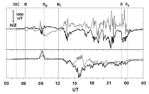
Figure 11. Variations in H / Z geomagnetic filed components in the interval, shown in Figure 9, recorded at ~ 30° to the east of the YeKB-radar field of view at the magnetic observatories TIK (top) and YAK (bottom)

At 18:17 UT, DIK recorded the next SLE event with a depth of ~ –1350 nT. From that moment until 02:20 UT on March 18, the plot of φ' i (UT) shows only signals with V Di <0 coming from φ' =55.2–58.9°. This corresponds to 400–600 km ranges and currents flowing in the E layer [Berngardt et al., 2015]. The spatio-temporal dynamics of this structure, designated by number 4 in Figures 2, b , and 7, a , is shown on maps 9–12 in Figure 10. The comparison of characteristics of its related BS i signals with variations in the geomagnetic field and riometer absorption indicates that the number of scattered signal decreases during absorption peaks accompanying the western electrojet field enhancements as in the cases of horizontal structures discussed in Section 4. Figure 3 of [Jacobsen, Andalsvik, 2015] drawn for the 20–24° E shows that at 20:00–23:30 UT the center of the western electrojet was below 59° N ( ϕ′ <55 °).

6.    RESULTS

We have identified effects of the St. Patrick’s Day strong geomagnetic storm in characteristics of backscattered signals received by the YeKB radar, and have compared these effects with disturbances of the ionosphere, geomagnetic field, riometer absorption, and total electron content within its field of view. Let us outline the main results of our study.

• •    The initial storm phase, developed when the magnetosphere is exposed to compressed solar wind and interplanetary magnetic field, was accompanied only by an increase in the number of signals backscattered by ground (BS g signals). The weak response of the magnetosphere-ionosphere system to the increase in the solar wind ram pressure from ~ 8 to 18 nPa is explained by the fact that during the previous 8 days of low geomagnetic activity the magnetosphere became stable relative to external impacts [Bargatze et al., 1985; Sharma et al., 2005].

• •    During the first step of the main phase, SYM-H decreased to –101 at IMF B_z <0, and then increased to –38 nT at IMF B_z > 0. The YeKB-radar data show wavelike decreases in the minimum range of BS g signals and a series of signals of diminishing range scattered in the ionosphere (BS i signals). At the stage of the ring current amplification, the diminishing ranges of BS g signals that could be caused by traveling ionospheric irregularities, coincided in time with increases in auroral activity; at the stage of attenuation, with the increase in the solar wind ram pressure. The series of BS i signals of diminishing range attended the equatorward extension of the current system of magnetospheric convection and the transition of the YeKB-radar field of view from the throat sector to the sector of dusk convection cell.

• •    During the second step of the main phase, SYM-H decreased to –234 nT. The YeKB-radar field of view passed into the westward electrojet sector. High values of f o E s , TEC and riometer absorption fluctuations suggest that all observation instruments were in the zone of auroral precipitation. This is confirmed by the results obtained in [Jacobsen, Andalsvik, 2016; Le et al., 2016].

The convection field reached maximum values of ~ 1.4 mV/m for this storm at 13:00–15:00 UT and remained at the level of E c ≤0.6 mV/m until the end of the early recovery phase. Nevertheless, at 15:00– 16:30 UT, auroral stations recorded a decrease in the AE index from 1700 to 700 nT; and stations within the radar field of view, the absence of significant geomagnetic disturbances. This is explained by a substantial equatorward shift of the westward electrojet. In this interval, YAK ( ϕ′ ~57°) observed a strong enhancement of the westward electrojet; and the YeKB radar, a discrete structure formed by BS i signals, which passed under absorbing sporadic E layers and were scattered in the polar cap.

Further equatorward expansion of the precipitation zone and westward electrojet led to the disappearance of BS_g and BS_i signals. The latter re-emerged after the beginning of multiple enhancements of the westward electrojet within the YeKB-radar field of view, which concurred with the AE , PCN / PCS increases. The BS i signals were observed for 8 hours at the end of the second step of the main phase, in the early recovery phase, and in the first two hours of the late one. The signals were scattered in the E region of the ionosphere and had eastward Doppler velocities. This points to the relationship between them and plasma processes developing in the westward electrojet.

• •    Discrete horizontal BS i structures during the days before the storm and in its late recovery phase were received from a limited range of latitudes and did not go beyond ϕ′ = 60–70°. On the days under study, they were observed in the vicinity of the afternoon in the convection throat; near midnight, in the Harang discontinuity; and in the morning, in the westward electrojet. The width of the zone of FAEDIs creating these structures increased with increasing geomagnetic activity due to lowering latitude of its southern boundary.

• •    In all these cases, the number of BS i signals forming discrete structures decreased until their complete disappearance during SLEs occurring with an increase in the riometer absorption.

• •    The decreasing number of BS_g events in the main and early recovery phases of the St. Patrick’s Day storm was associated with the absorption, the level of which in the lower ionosphere increased due to impact ionization. In the late recovery phase of the storm, the number of BS g signals decreased due to changes in the composition of the neutral atmosphere. This conclusion follows from the analysis of TEC data and is confirmed by the analysis of the [O]/[N 2 ] ratio, carried out for this storm in [Astafyeva et al., 2015].

The work was supported by the RF President Grant of Public Support for RF Leading Scientific Schools (NSh-6894.2016.5) and partially by the RFBR grant No. 14-05-00588.