Discrete Model of Commensalism Between Two Species

Published Online August 2012 in MECS DOI: 10.5815/ijmecs.2012.08.06

Mathematical modeling is an important interdisciplinary activity which involves the study of some aspects of diverse disciplines. Biology, Epidemiology, Physiology, Ecology, Immunology, Bio -economics, Genetics some of those disciplines. This mathematical modeling has raised to the zenith in recent years and spread to all branches of life and drew the attention of every one.

Mathematical modeling of ecosystem was initiated by Lotka[1] and by Volterra[2]. Since then, several mathematicians and ecologists May[3], Kushing[4], Smith[5], Kapur[6], contributed to the growth of this area of knowledge.

Competitive eco-systems of two species and three species with limited and unlimited resources were investigated by Srinivas[7] while Laxminarayan and Pattabhi Ramacharyulu[8] studied Prey-Predator ecological models with partial cover for the prey and alternate food for the predator. Archana Reddy[9] and Bhaskara Rama Sharma[10] investigated diverse problems related to two species competitive systems with time delay. Further Phani Kumar[11] studied some mathematical models of ecological commensalism. More recently the criteria for a four species syn eco-system was discussed at length by the present authors[12-20].

The present investigation is a study of discrete model of commensalism between two species. Figure 1 shows the schematic sketch of the system under investigation.

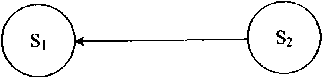
Commensal of S2 (Gets benefit from S2)

Host of Si

(Not effected by the interaction with S;)

Figure 1: Schematic sketch of the system

Commensalism is a symbiotic interaction between two populations where one population (S₁) gets benefit from (S₂) while the other (S₂) is neither harmed nor benefited due to the interaction with (S₁). The benefited species (S₁) is called the commensal and the other (S₂) is called the host. Some real-life examples of commensalism are presented below.

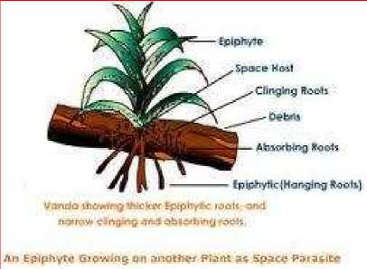
Figure 2. Example for commensalism

• 1.    Epiphytes are small green plants found growing on other plants for space only. They absorb water and minerals from the atmosphere by their hygroscopic roots and prepare their own food. The plants are not harmed in any way. This is shown in Figure 2.

• 2.    A squirrel in an oak tree gets a place to live and food for its survival, while the tree remains neither benefited nor harmed.

• 3.    The clownfish shelters among the tentacles of the sea anemone, while the sea anemone is not effected

• II.    BASIC EQUATIONS

The model equations for two species host-commensal is given by the following system of first order non-linear differential equations employing the following notation.

Notation Adopted :

N1(t): The population strength of commensal species (S1)

N2(t): The population strength of host species (S2)

t : Time instant ai     : Natural growth rates of Si, i = 1, 2

a ii      : Self inhibition coefficient of S i , i = 1, 2

a 12     : Commensal coefficient of S 1 due to S 2

K i = a ⁱ : Carrying capacities of S i , i = 1,2 a ii

Further the variables N1, N2 are non-negative and the model parameters a1, a2, a11, a12, a22 are assumed to be non-negative constants.

The basic model equations for the growth rates of S 1 , S 2 are

N i (t+1)=N i (t),i=1,2                 (6)

• i)    Fully washed out state.

E o : N ₁ = 0 , N ₂ = 0

• ii)    The state in which only the host (S₂) survives and the commensal (S₁) is washed out.

E 1 : N ₁ = 0 , N ₂ = K ₂

• iii)    The state in which the commensal (S₁) only survives and the host (S₂) is washed out.

E 2 : N = K ₁ , N₂ = 0

• iv )    The Co-existent state (or) Normal steady state.

Е з : N ₁ = K ₁ + bi K² , N = K ₂ a ₁₁

• IV.    STABILITY OF THE EQUILIBRIUM STATES

The basic equations can be linearized about the equilibrium point E(N1 , N2 ).We get the characteristic matrix is given by a 1 - 2a11N1 + a12N2

a 12 N 1

a ₂ - 2a₂₂N₂

The equilibrium point E (N1,N2) is stable, if the absolute values of all eigen values of the matrix A are less than one.

—¹ = a. N - a_u N 2 + a_n N, N,        (1)

1      1        11     1         12      1      2

dt

4.a. Stability of equilibrium point E0

The characteristic matrix of this state is dN2 dt

= a ₂ N ₂

-

a ₂₂ N ₂

A =

a 1 + 1

^a2 ^{+ 1}

The discrete form of the equations (1) and (2) is

N i (t)= a i N i (t-1)-a_n N ? (t-1)+a i2 N i (t-1)N 2 (t-1) (3) N 2 (t)= a 2 N 2 (t-1 )-a 22 N 2 (t-1) (4) where a ₁=a₁+1 and a ₂ a₂+ 1 (5) III. EQUILIBRIUM STATES

The system under investigation has four equilibrium points defined as

The eigen values of which are a1 + 1, a2+ 1 and the absolute values of these both are greater than one.

Hence, E₀ (0, 0) is unstable.

4.b. Stability of equilibrium point E1

The characteristic matrix is state is a1 + a12K2 + 1    0

0        1 - a₂

The eigen values of which are a1+ a12 K2 +1, 1-a2. Since, absolute value of one of the two eigen values is greater than one.

Hence, E 1 (0, K 2 ) is unstable .

4.c. Stability of equilibrium point E2

The characteristic matrix in this state is

results are illustrated in Figures 3 to 12 and the observations are presented below.

Results and Observations

A =

1 — a10

a 12 K 1

^a2 ^{+ 1}

(10)

The eigen values are 1 – a 1 , a 2 +1

Since, absolute value of one of the two eigen values is greater than one.

Hence, E 2 (K 1 , 0) is unstable.

4.d. Stability of equilibrium point E3

The characteristic matrix of this state is

A =

Га.) i-(a+ a к) a„ K+a2 K

V      ^а11    )

0              1-a2

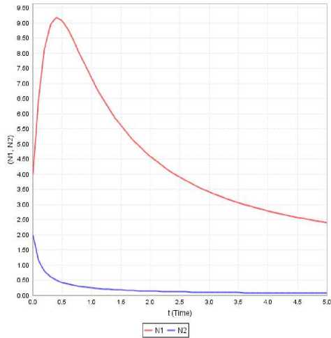
Figure 3: Variation of N₁ and N₂ against time(t) for

The eigen values are

a 1 =0.144, a 11 =0.232, a 12 =4, a 2 =0.144, a 22 =3.786, N₁₀=4, N₂₀ =2

1 — (a1 + a12 K2) and 1 — a 2

Case (i) : When (a₁ + a₁₂ K₂) < 2 and a₂< 2

The absolute value of both the eigen values is less than one.

Hence, the equilibrium point E 3 ( N 1 , N ₂ ) is stable.

Case (ii) : When a₁ + a₁₂K₂= 1 and a₂= 1

The absolute value o f b o th the eigen values is less than one. Hence, E 3 ( N 1 , N ₂ ) is stable.

Case (iii) : When a 1 + a₁₂ K₂ >  2 or a₂ >  2 or both >  2

The absolute value of one of the two eigen values or both the eigen values is greater than one. In this case,

E 3 ( N 1 ,N 2 ) is unstable.

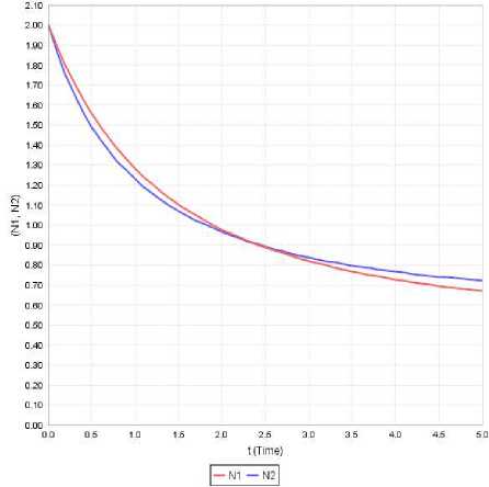
Figure 4: Variation of N₁ and N₂ against time(t) for a 1 =0.125, a 11 =0.906, a 12 =0.567, a 2 =0.345, a 22 =0.543, N 10 =2, N 20 =2

• V.    A NUMERICAL APPROACH OF THE GROWTH RATE EQUATIONS

The numerical solution of the growth rate equations (1) and (2) computed emplo ying the fourth order Runge-Kutta method for specific values of the various parameters that characterize the model and the initial conditions. For this MATLAB has been used, the

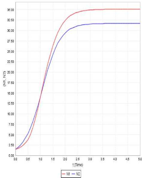
Figure 5: Variation of N₁ and N₂ against time(t) for a 1 =1.068, a 11 =0.868, a 12 =4, a 2 =0.928, a 22 =2.788, N 10 =1.5, N 20 =1.5

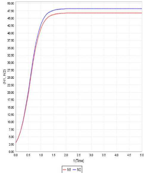
Figure 7: Variation of N₁ and N₂ against time(t) for a 1 =4.685, a 11 =0.26, a 12 =0.155, a 2 =4.82, a 22 =0.1, N₁₀ =3, N₂₀ =3

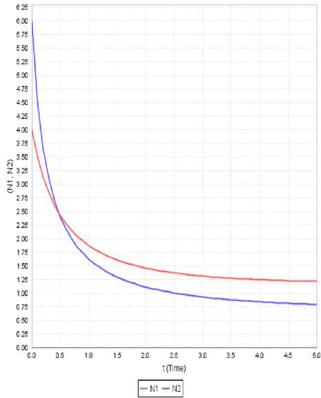
Figure 6: Variation of N₁ and N₂ against time(t) for a 1 =0.753, a 11 =0.714, a 12 =0.12, a 2 =0.455, a 22 =0.633, N 10 =4.5, N 20 =6

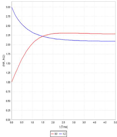
Figure 8: Variation of N 1 and N 2 against time(t) for a 1 =0.405, a 11 =0.65, a 12 =0.515, a 2 =1.075, a 22 =0.515, N₁₀ =1, N₂₀ =3

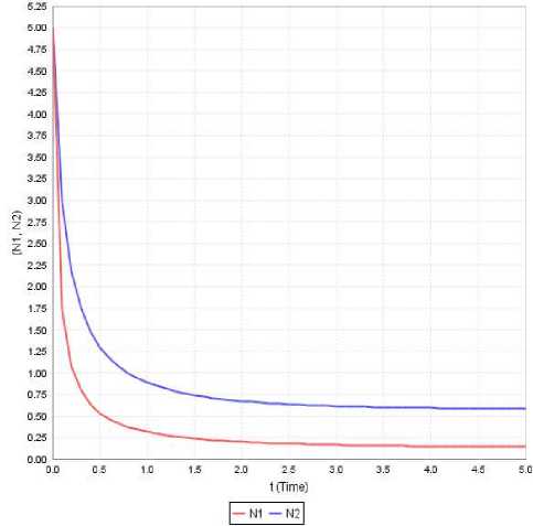
Figure 9: Variation of N₁ and N₂ against time(t) for a 1 =0.405, a 11 =4.395, a 12 =0.305, a 2 =0.94, a 22 =1.615, N 10 =5, N 20 =5

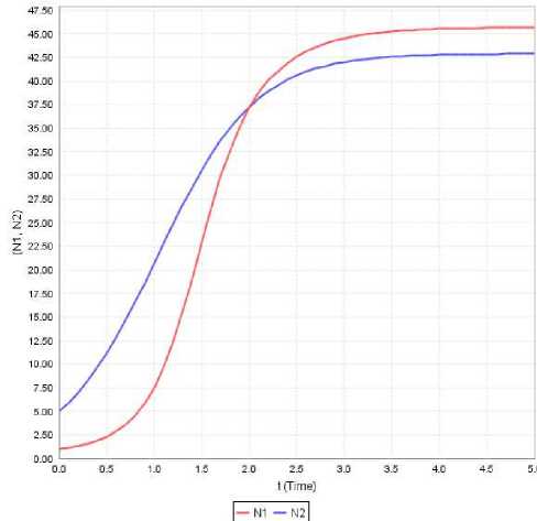
Figure 11: Variation of N₁ and N₂ against time(t) for a 1 =0.91, a 11 =0.142, a 12 =0.13, a 2 =1.956, a 22 =0.046, N 10 =1, N 20 =5

(N1, N2)

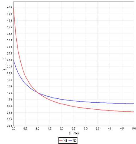
Figure 10: Variation of N 1 and N 2 against time(t) for

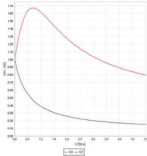
Figure 12: Variation of N 1 and N 2 against time(t) for a 1 =0.21, a 11 =0.927, a 12 =2.844, a 2 =0.189, a 22 =1.923, N₁₀ =1, N₂₀ =1

a 1 =0.144, a 11 =0.896, a 12 =0.304, a 2 =0.648, a 22 =0.792,

N 10 =4.5, N 20 =2.5

Figure 13: Variation of N1 and N2 against time(t) for a1 =0.230, a11 =1.490, a12 =1.460, a2 =0.190, a22=1.40, N10 =5, N20 =10

Observations of the above graphs

Case-i: In this case the first species would always dominates the second species. Further the first species has a steep rise and later falls at a very low rate. The second species decreases initially and in course of time it is almost extinct as seen in Figure 3.

Case-ii: In this case initial strength of both the species is same and the first species dominates over the second species till the time instant t*=2.4 and thereafter the dominance is reversed. Further both the species maintain steady variation with low growth rates as seen in Fig 4.

Case-iii: In this case initial strength of both the species is same and the second species dominates over the first species till the time instant t*=1 and thereafter the dominance is reversed. Further we notice that both the species have a steady variatio n with no appreciable gr o w t h r a t e s. This is illustrated in Figur e 5 .

Case-iv: In this case initially the second species dominates over the first species till the time instant t*=0.45 and thereafter the dominance is reversed. It is evident that both the species asymptotically converge to the equilibrium point. Further both the species maintain steady variation with low growth rates as seen in Fig 6.

Case-v: In this case initial strength of both the species is same and the second species would always dominate over the first species. Further we notice that both the species have a steady variation with no appreciable growth rates. This is shown in Figure 7.

Case-vi: In this case initially the second species dominates over the first species till the time instant

t*=1.5 and thereafter the dominance is reversed. Further we see that the first species rises initially and later maintains a steady variation with no appreciable growth rate. Where as the second species decreases initially and in course of time it is almost extinct as seen in Figure 8.

Case-vii: In this case initial strength of both the species is same and the second species would always dominate over the first species. It is evident that both the species asymptotically converge to the equilibrium point. Further both the species maintain steady variation with low growth rates as seen in Figure 9.

Case-viii: In this case initially the first species dominates over the second species till the time instant t*=1 and thereafter the dominance is reversed. It is evident that both the species asymptotically converge to the equilibrium point. Further both the species maintain steady variation with low growth rates as seen in Fig 10.

Case-ix: In this case initially the second species dominates over the first species till the time instant t*=2 and thereafter the dominance is reversed. Further we notice that both species have a steady variation with no appreciable growth rates. This is shown in Figure 11.

Case-x: In this case initial strength of both the species is same and the first species would always dominates the second species. Further the first species has a steep rise and later falls at a very low rate. The second species decreases initially and in course of time it is almost extinct as seen in Figure 12.

Case-xi In this case initially the second species dominates over the first species till the time instant t*=0.2 and thereafter the dominance is reversed. Further the first species has a steep rise and later falls at a low rate. It is evident that both the species asymptotically converge to the equilibrium point as shown in Figure 13.

• VI.    CONCLUSION

The present paper deals with the study on discrete model of commensalism between two species. The model comprises of a commensal (S1), a host (S2) that benefit S1, without getting effected either positively or adversely. Al the four equilibrium points are identified based on the model equations. The model would be stable, if each of the eigen values is numerically less then one. It is observed that, in all four equilibrium states, only the coexistent state is stable when

• (i)    ( a 1 + a ₁₂ K 2 ) <  2 and a 2 <  2
  
  ⁽ⁱⁱ⁾    ( a 1 + a ₁₂ K 2 ) = 1 and a 2 = 1

Acknowledgment

We thank to Prof..M.A.Singara Chary,Head, Dept.of Microbiology, Kakatiya University, Warangal, (A.P), India and Prof. C. Janaiah Dept. of Zoology, Kakatiya University, Warangal (A.P), India for their valuable suggestions and encouragement. And also we acknowledge to Mr.K.Ravindranath Gupta for neat typing of this research paper.