Discrete wavelet transform based high performance face recognition using a novel statistical approach

Published Online June 2018 in MECS DOI: 10.5815/ijigsp.2018.06.01

Contemporary life has brought people in fascinating comfort and convenience as well as vital challenges that are to be concerned with cautiously. Technological improvements and accordingly potential applications are just limited by people’s imagination. Changing sociocultural structure due to evolving technological lifestyle has led to the emergence of new security problems. Crime rate increases day by day very quickly. The success rate of crime prevention can be enhanced by the implementation of technology again.

Crime prevention can be maintained in two ways;

• -    Detecting and weeding out criminals in public environments: Recognizing the criminals in dynamic environments among thousands of people in seconds is a challenging task. Making multiple searches simultaneously, such as trying to identify multiple criminals from thousands of people at an airport or train station is not something that can be done by manpower.

• -    Identity forge prevention: As the variety of transactions and applications that computers are integrated into our lives have increased dramatically, authorization of individuals for valid enrollment has become vital. Even banking transactions, military applications, cellular phone devices, computers, building and room entrances, etc. all require identity verification [1-2]; all these applications are still seriously vulnerable to frauds such as identity forge [3].

The most reliable way of identifying an individual whether it is genuine or not is analyzing its biometrics such as the face, fingerprint, iris, ear, handwriting, etc. [4]. Biometrics refers to the identification of individuals based on their physiological and/or behavioral characteristics [5]. These body markers are unique for each individual, which facilitates them to be used confidentially for authentication [6]. Besides, there is no case like an iris or fingerprint of an individual being stolen or forgotten as password information. Biometric systems can be used in two ways [7]; identification- the identity of an individual is determined; verification- the claim of an identity is verified and accordingly is accepted or rejected.

FR is one of the prominent biometrics encompassing superiorities regarding other traits such as being able to capture at a distance in a friendly manner, as well as some drawbacks like being computationally complex [89]. Though many research studies have been proposed in the literature, FR still embodies considerable challenges such as facial expression, poses, and illumination [9-12]. Feature extraction and classification form the basis of FR. An efficient representation of the face must be achieved by extracting ideal features from the image to reduce the computational complexity and increase the classification accuracy [13]. Classification is the verification of an individual according to those features by deciding whether it belongs to a particular class or not. Thus, development of computation-cost-friendly feature extraction and classification methods is crucial [9, 14].

For feature extraction, which is the epicenter of FR, many methods (Linear Discriminant Analysis (LDA) [15], Principle Component Analysis (PCA) [16], Linear Binary Pattern (LBP) [17], Gray-level Co-occurrence Matrix (GLCM) [18]) have been utilized and their performances have been analyzed.

Wavelet transform has gained great interest in computer vision and image processing especially in the areas such as compression and recognition regarding its advantages like multi-resolution and space-frequency resolution [9]. Wavelet transformation decomposes the image into different sub-bands that is similar to the operation of the human visual system which makes it preferable for the textual retrieval, segmentation, and classification [13, 19-27].

In this study, we present a high-performance FR architecture that is a combination of signal-based and statistical approaches. The proposed architecture mainly based on DWT and a novel textual feature extraction method GLTDM which holds statistical information about the Discrete Wavelet Transform (DWT) of the original face image. GLTDM utilizes the orientational relationships of the same pixel patterns occurring at different positions in an image rather than their occurrence statistics as applied in GLCM-based counterparts. The approximation and three detail subbands of the images are first calculated. GLTDMs specific to these four matrices are subsequently generated. The Haralick features are extracted from the generated four GLTDMs. At the following stage, a joint feature vector is formed using these four groups of Haralick features. Lastly, extracted features are classified by using K-NN algorithm. As demonstrated in the simulation results, the proposed approach performs promising results and outperforms other classical methods in the context of classification.

The rest of the paper is organized as follows. Section II introduces preliminary information about GLCM, Haralick features, and DWT. Section III proposes the GLTDM and utilization of it with DWT for FR. Section IV presents the simulation results and discussions. Lastly, Section V concludes the paper.

• II.    Preliminaries

In this section, we give an introductive explanation for GLCM, Haralick Features, and DWT subsequently, which we believe would be useful to better cover the methodology we propose. The first part presents the calculation steps of GLCM which is subsequently followed by the presentation of the fourteen Haralick features and the last part finalizes the section with a summary of DWT.

• A.    GLCM

Texture can be defined by regular or random patterns that repeat over a region and is one of the important characteristics used in identifying regions or objects of interest in an image [18, 28-29]. Spatial distribution of gray levels in a neighborhood defines the texture of an image. Texture analysis has become very important especially in machine vision tasks such as scene classification, shape determination, object recognition [30] which led to gain a wide application area ranging from medical imaging to remote sensing [31].

A great deal of work has been proposed about texture analysis in the literature. These methods can mainly be categorized as parametric-model based approaches, geometrical approaches, signal-processing approaches and statistical approaches.

Statistical approaches are the simplest methods applied for texture description of an image or a region in the image. The most basic way is utilizing the statistical moments of the intensity histogram [32-33]. Statistical approaches utilize the first, second, etc. order of statistics of distributions of pixels with particular gray-level patterns and orientations in the image [34].

Let z expresses an intensity value between 0 and L-1 (for 8-bit unsigned integer representation L=256 ), p(z i ) , ( i=0,1,2,...,L-1 ) is the histogram of the corresponding image. n^th moment of z about the mean intensity value is calculated as follows:

^ n ^(z) = Z^z - m)^u p(z_t)         (1)

where m expresses the mean intensity and is defined as:

m = Z0"1zip(zi)               (2)

Obviously, the first ( µ 0 ) and second ( µ 1 ) order moments are equal to 1 and 0 respectively. The second order moment ( u₂ ) denotes the variance ( o(z) ) which gives a deterministic idea about the texture of an image. For example, variance ( o(z) ) is smaller for the regions that encompass lower changes in intensity values and converges to 0 for constant intensity values. Texture analysis by means of inspecting only the histogram data does not give decisive information about the spatial relationships of the pixel values with each other [32-33].

GLCM is one of the prominent statistical feature extraction and analysis approach that, a lot of research studies have based on [35]. GLCM incorporates also the spatial relationships of intensity values with each other as well as their occurrence quantities. Let f is an image whose intensity values vary in the interval [0, L-1]. Each element of GLCM indicates the number of times that the pixel pair (zi, zj) occurred in f with orientation Q. The orientation represented with Q eventually represents a displacement vector d=(dx,dy | dx=dy=dg) where dg is the number of gaps between the pixels of interest. For the situation of adjacency dg=0. Orientation can also be represented by two parameters as the distance d that the intensities zi, zj apart from each other with angle α [3637]. d can take values between 0 and L-2 theoretically. The orientation of the pixel pattern can be at four different directions as 0°, 45°, 90° and 135° that α can take. That is, each image can have four different GLCMs for each angle (0°, 45°, 90° and 135°) for a specific d. The size of a GLCM depends on the discrete intensity values in the image. If the intensity values of the image vary in the interval [0, L-1] then the size of the GLCM becomes (L-1)×(L-1). An example of the configuration of the four GLCM matrixes (GLCM0°, GLCM45°, GLCM90°, GLCM135°) of an image f for d=0 is demonstrated in Fig. 1.

GLCM 135°

2	2	1	0	0	1	0	1
1	2	3	1	1	0	2	0
3	2	1	2	0	2	1	0
1	2	2	0	1	0	0	0
1	1	1	0	0	1	1	0
0	1	1	2	2	0	0	0
0	0	1	0	2	1	0	0
0	0	0	0	0	0	0	0

GLCM 90°

2	2	3	2	0	0	1	0
3	1	2	1	1	1	0	1
1	2	3	1	1	3	2	0
0	4	0	1	1	0	0	0
2	0	1	1	1	0	1	0
1	1	1	1	2	0	0	0
0	1	1	0	1	1	0	0
0	0	0	0	0	0	0	0

3	5	4	3	2	5	8	4
1 1	5	6	6	7	3	2	1
	4	6	7	1	3	4	5
5	5	3	3	2	1	4	6
6	7	7	3	2	1	2	2
3	3	5	2	1	2	1	4
1	2	2	4	6	3	2	3
3	3	4	1	3	5	6	3

GLCM 45°

1	1	2	2	2	1	0	0
1	3	1	2	1	1	0	0
2	4	1	0	0	0	3	1
2	0	0	1	1	1	0	0
0	1	1	2	0	1	0	0
0	2	2	0	1	1	0	0
0	0	2	0	1	0	1	0
0	0	0	0	0	0	0	0

0	3	2	3	1	0	0	0
5	2	1	1	1	0	0	0
0	5	3	2	3	0	0	0
1	0	1	0	1	3	0	0
0	1	1	1	1	2	0	1
0	0	2	0	0	1	3	0
1	0	2	0	0	0	1	0
0	0	0	1	0	0	0	0

GLCM 0°

Fig.1. The configuration of GLCMs of an image f for d=0 .

• B.    Haralick Features

Haralick [33] proposed 14 features that can be extracted from the abovementioned GLCM_a ° matrices. There are two ways of obtaining the Haralick features from the four GLCMs of an image. The first method is calculating the average GLCM matrix of the image according to Eq (3) and subsequently extracting features from that average GCLM matrix [18, 38-39].

GLCM_avg = (GLCM₀ ° + GLCM 45 + GLCM₉₀ ° + GLCM-J/A (3)

The second way is finding angular types of each feature and later calculating the average of each as follows:

f_u avg = (/_n o- + /_n 4S" + /_n 90- + /_n i3s- )^/4 ⁽⁴⁾

where fnavg represents the average value of an arbitrary Haralick feature, and fno°, fn4s°, fn9o°, fni3s° express the angular constituents of the average feature value respectively. Haralick claimed that each of these 14 features gives hints about some textual characteristic of an image. For example, a higher value for the entropy feature of an image implies the level of the complexity of the image. The less random an image is, the higher uniformity and contrast tend to be. Besides, the higher probability values near the main diagonal stands for the images with rich gray levels that represent the areas with slowly varying intensity levels [35]. The list of 14 Haralick features [1, 20, 33] are given in Table 1.

Table 1. Haralick features.

Angular Second Moment	f 1=T. t a1S^1P(ij)2
Contrast	h    y : - .'' p 2 {L'xy' j - 1 P4,j)}  ^
Correlation	f     V N s jjN« (i~Px')(i-Py')(P(i,j') Г з     S i=1 S j=1       Т х Т у
Sum of Squares	f 4=x’ ! =iS^1(l-V)2P(lJ)
Inverse Difference Moment	f s = Sj^ 11+(1_n2 P(i,j)
Sum Average	f 6 = !. 2” а 2 1Р х + у (1)
Sum Variance	f 7 = I. 2 i j 2 (i-f8) 2 P x + y (i)
Sum Entropy	f8 = —Y.^ P x+y(i) lOg{P x+y(i) }
Entropy	f9 = - 2 i Y j P(i,j)log{P(i,j)}
Difference Variance	f10 = variance of px-y
Difference Entropy	f 11 = -Y'ja 2 1 P x-y (Q^Og{P x-y(Q}
Information Measures of Correlation	_ HXY-HXY1 f 12 = max {HX, HY{ f13 = (1 - exp[-2.0(HXY2 - HXY){Y /2 HXY = -Y i !. j p(i,j)togp(i,j)
Maximal Correlation Coefficient	РУИти*) vk-,j)     Lк т х (Г)р у (к) f14 = (Second Largest Eigenvalue of Q{ 1/2

where:

N_g : The number of discrete intensity levels in the quantized image

p(i,j) : (i,j) th entry in the normalized GLCM matrix p_x(i), P y (j): i th entry in the marginal-probability matrix

P x ⁽ⁱ⁾ = Z^PGJ) , PyU) = Z^P^A P x+ _y(k) = $^(.i,D,k = 2,3, _2N_g }_|i+._|=fe

P x-y ⁽k⁾ = ^{I.^ i ^S^ i P^(i,j),k = 0,1, ™^,N_g ^{- 1}}_ц__у|=(£

HX and HYare the entropies of p_x and p_y respectively that are calculated as follows:

^HX = -Z^Px® ¹°9{РхО

^HY = ^-S^ i P_y^(j) ^l°g{P y (j")} '■   N_g

HXY1 = - H P(i,j) 1од{рх(0Ру(Л} i=1 j=1

N g N g

H XY2 = - zz P x (ⁱ)P y (^j) log{p_x(i)P y (B} l=1 j=1

• C.    DWT

Generally, signals are represented in the timeamplitude domain on a two-dimensional axis which expresses the altitude of the signal at each moment. However, sometimes much more valuable deterministic information is hidden in the frequency content of the signal. That is, the required information may be better seen or analyzed in the frequency domain, i.e. in image processing, some types of noise are better filtered in the frequency domain. Fourier Transform (FT) expresses the signal at frequency-amplitude domain by breaking the signal into sine waves of different frequencies. These frequency components comprise the frequency spectrum which identifies what frequencies exist in the signal. However, FT gives only the frequency components of the signal, no more than. Sometimes, it is required to know the time localization of particular spectral components of the signal. That is to determine at which intervals the particular components occur. Wavelet transformation (WT) gives the frequency-time representation of the signals [40-41]. Besides providing the frequency-time representation, WT has some advantages over FT such as providing better approximations for the signals with sharp peaks and discontinuities [42] which is also beneficial especially for discrete-time signals that are described by piecewise polynomials like images [43].

Essentially, DWT yields the analysis of a signal at different frequency bands at different resolutions by decomposing into its approximation and detail components [40]. For the DWT of an image which is a two-dimensional (2D) signal, three 2D wavelets (^H(x,y), ^v(x,y),  ^D(x,y)) and a scaling function (ф(х,у)) is required that are associated with high-pass and low-pass filters respectively. Four of the products of these 2D functions are again 2D and they constitute the separable scaling function and directionally sensitive, separable wavelets as follows [32]:

ф(х,У) = ф(х)ф(у)(5)

^н(х,у) = ^(х)ф(у)

^v(x,y) = ф(%Жу)

грп(х,у) =гр(х)гр(у)(8)

where ^H (x,y),  ^v(x,y), yD (x,y) measures intensity variations in the images along horizontally, vertically and diagonally respectively.

The DWT of an image with the size MxN is calculated as follows:

W>(j.^m.ⁿ⁾ = — У^-; У^- \ПхУ)ЧфУ⁽Уу)1 ¹ = ^{H, V,D^} (10) where

Ф j,m,n (х,y') = 2^j/'^zф(2^jх - m, 2^jy — n) (11)

^ j,m,n (x,y) = 2^j/2^^l(2^jx —m,2^jy — n) i = {H,V,D} (12)

W p (j₀, m, n) and W ^ (j, m, n) coefficients express the approximation of image f(x,y) at scale j₀ and horizontal, vertical, diagonal details for scales j >  j₀ [32].

DWT starts with applying a half-band low-pass filter to the original signal and concludes with a down-sampling operation. That is passing the frequency components that are lower and equal than the highest frequency component of the signal. The remaining part is the approximation part, which is comprised of the low-frequency components encompassing the essential information. The rest is the high-frequency components holding the detail parts such as edges, contours, etc. Fig. 2-4 depict the operational block diagram of 1-D and 2-D DWT respectively [32, 40, 42, 44]:

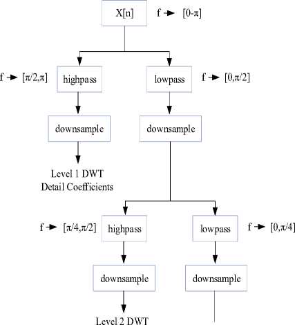
Detail Coefficients

Fig.2. 1-D wavelet transform.

W ,^D (j,m,n) (HH)

W (j, m, n) (HL)

W ф (j+1,m,n)-

^W< pUo ^,m,n) = ^Хх^Х^ О f⁽X^,У')ф j₀, _m , _n⁽X^,y) ⁽⁹⁾

W ф (j,m,n) (LL)

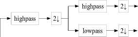
Fig.3. 2-D wavelet transform.

LL	HL	HL
LH	HH
LH		HH

Fig.4. 2-D wavelet transform demonstration.

where,

2↓: states the down-sampling operation,

• LL: (low-frequency part of both horizontal and vertical direction) – approximation component,

LH: (low-frequency part of the horizontal direction, high-frequency part of vertical direction) – vertical details

HL: (low-frequency part of the vertical direction, high-frequency part of horizontal direction) – horizontal details HH: (high-frequency part of both horizontal and vertical direction) – diagonal details [44].

• III.    Proposed Methodology

In this study, we propose a novel FR approach, that mainly basis on DWT and GLTDM that is inspired from GLCM but a better feature extraction method and joint feature vector formation processes. Obviously, the strength of the classification is significantly identified by how deterministic the features extracted from the image are. DWT of the image ( f(x,y) ) is given to the GLTDM calculation to develop more deterministic features, rather than its original format. As a result of DWT step, four sub-images (LL, HL, LH, HH) are generated. Following this stage, each of these sub-images is applied to the GLTDM formation process as an input.

As mentioned in the previous section, GLCM is one of the prominent and simplest statistical feature extraction and analysis approaches [38-39]. Image histograms provide information about just the intensity distributions in an image. However, the more deterministic idea can be obtained about the texture of an image by examining the relative positions of the intensity values in the image which is provided by GLCM. GLCM provides statistics about the occurrences of particular pixel patterns in the image depending on their orientation and distances as mentioned above.

In this study, we propose an alternative feature extraction method GLTDM that considers more detailed spatial relationships of the pixel patterns. By this way, much more distinguishing features are formed that ultimately increases the classification that is FR performance.

We generate a GLTDM matrix that holds the total displacement information for the occurrences of pixel pairs in the image. The total displacement for all occurrences of a pixel pair (zi, zj) in the image is calculated as follows:

GLTDM(Z i ,Z j ) = 2™^C 1 ^(Z ‘ ^,Z,) V(^ m - X m-1 ) 2 + (У т — У т-1 )² (13)

where x m and y m express the row and column indices of the pattern in the image respectively.

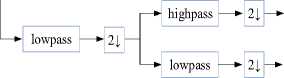
Let consider the image f MxN given in Fig. 2, which encompasses pixels with eight distinct gray levels. For the orientation Q ( d =0 , a=0° ), the total displacement for pixel pair (z_i=3, z j =2) is calculated as totaldisp ( _1,1 ) = (d 1 +d 2 +d 3 +d 4 +d 5 ) as depicted in Fig. 5:

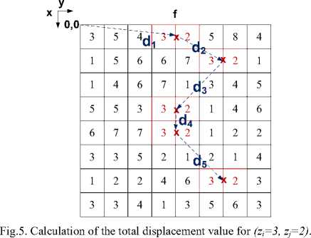
GLTDM matrices for different a variations of the sample image f (Fig. 1) are illustrated in Fig. 6:

0	13	11	10	2	0	0	0
15	14	10	8	5	0	0	0
0	13	10	13	10	0	0	0
9	0	3	0	8	13	0	0
0	7	4	2	4	10	0	6
0	0	11	0	0	4	9	0
5	0	9	0	0	0	5	0
0	0	0	7	0	0	0	0

8	9	11	8	3	9	0	0
7	12	6	12	7	9	0	0
9	15	9	0	0	0	9	6
13	0	0	9	8	4	0	0
0	10	7	5	0	4	0	0
0	10	11	0	5	4	0	0
0	0	6	0	5	0	5	0
0	0	0	0	0	0	0	0

(a) GLTDM 0°             (_b) _GLTDM45°

9	11	8	0	0	6	0	8
9	10	12	9	7	0	9	0
17	13	6	9	0	8	7	0
4	15	9	0	8	0	0	0
4	9	3	0	0	10	7	0
0	9	11	9	5	0	0	0
0	0	5	0	6	5	0	0
0	0	0	0	0	0	0	0

9	10	13	15	0	0	6	0
10	7	9	9	8	9	0	7
8	13	15	11	6	12	8	0
0	16	0	8	4	0	0	0
16	0	10	4	3	0	7	0
9	11	4	4	16	4	0	0
0	5	6	0	5	5	0	0
0	0	0	0	0	0	0	0

(c) GLTDM 90°            (d) GLTDM 135°

Fig.6. Configuration of the GLTDM of an image for d=0: (a) GLTDM 0° , (b) GLTDM 45° , (c) GLTDM 90° , (d) GLTDM 135° .

As in GLCM, four GLTDMS are generated for each direction, 0°, 45°, 90° and 735° that a can take. However, since DWT of the image is given to feature extraction rather than itself, four input sub-images are applied (LL, HL, LH, HH) . As a result, four GLTDMs are formed for a single direction a and totally sixteen for all.

Considering a single direction a , features are extracted from each GLTDM of (LL, HL, LH, HH) sub-images. Fourteen Haralick features are extracted from each GLTDM. Following this stage, these features are concatenated to form a Joint Feature Vector (JFV). Eventually, JFV is comprised of 56 features. The ultimate JFV is given subsequently to the classifier. K-NN algorithm (45-46) is utilized for the classification process.

The operational block diagram of the methodology is demonstrated in Fig. 7:

Face Database

LL

GLTDM(LL) α

Face Image

f(x,y)

DWT

HL

LH

GLTDM generation

HH

GLTDM(HL) α

GLTDM(LH) α

Scale

GLTDM(HH) α

Scaled GLTDMs

Feature Extraction

Haralick Features(LL) Haralick Features(HL) Haralick Features(LH) Haralick Features(HH)

Feature Concatenation

JFV

Classification (K-NN)

Fig.7. Operational block representation.

• IV.    Simulation Results and Discussions

We use the faces94 [47] face database to test the performance of the proposed method. Experiments are implemented by using 200 images per 152 distinct individuals, including frontal views of faces with different facial expressions, each of size 64 x 64 pixels obtained from faces94 color image database as shown in Fig. 8. To describe the properties contained in the cooccurrence matrices, we used 14 statistical measures that are computed from the matrices: angular second moment, contrast, correlation, sum of squares, inverse difference moment, sum average, sum variance, sum entropy, entropy, difference variance, difference entropy, two information measures of correlation, and maximal correlation coefficient. Once the features are extracted from each sub-images, we used the concatenation strategy to combine them in a manner to take advantage of the multiple scale information.

Features extracted from GLCM are combined into a single feature to form JFV. For all experiments,the nearest neighbor classifier is applied for all variables. Randomly selected 15 images of each person are used for training and the remaining images are applied for testing. The train-test splits are repeated 10 times for statistical significance, and average recognition rates are reported. We have evaluated the number of intensity levels, symlet approaches to determine how various values differ results, and strategy for combining the feature descriptors extracted from different sub-images. Texture classification results achieved by multiple a descriptors for different symlet values are presented in Table 2. It can be easily seen that the best classification performance for a=0 ° belongs to sym-12 for intensity level L=16 whereas sym-12 achieves the highest classification rate for every intensity value for a=45 ° a=90 ° and a=135 ° in Table 2.

Table 2 and Figure 9 identify that sym-12 has better classification performance than sym-4 and sym-8 which reveals the fact that classification performances of the methods mainly depend on the wavelet decomposition structure. The direction of DWT for α values is the other deterministic factor that affects the classification performance. Directions a=90°and a=135 ° have better performances than other directions for sym-12. Despite the raise in the classification performance regarding an increase in the symlet values, decomposing with symlet values higher than 12 is unnecessary which increases the run-time and complexity. Because symlet 12 has 0.99 performance for almost every intensity level and a values.

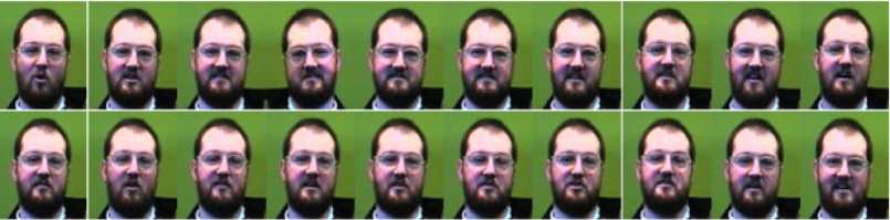
Fig.8. Examples of face images extracted from faces94 [47] face database.

Table 2. Texture classification results achieved by multiple α descriptors for different symlet values. The results show the classification rates on percentage.

	a=0°				a=45°								a=90°			a=135°
	16	32	64	128	256	16	32	64	128	256	16	32	64	128	256	16	32	64	128	256
Sym-4	0.86	0.8	0.9	0.82	0.84	0.82	0.82	0.8	0.76	0.80	0.82	0.82	0.8	0.82	0.8	0.80	0.8	0.8	0.78	0.80
Sym-8	0.90	0.94	0.90	0.86	0.94	0.90	0.86	0.9	0.94	0.82	0.94	0.92	0.92	0.96	0.88	0.86	0.86	0.86	0.86	0.86
Sym-12	0.96	0.90	0.94	0.86	0.86	0.96	0.98	0.99	0.96	0.98	0.99	0.99	0.99	0.98	0.98	0.96	0.98	0.99	0.96	0.96

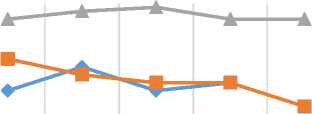
Classification performance of GLCM, GLTDM, and DWT with sym-12 are compared for direction 135. There are important observations that can be made according to the results shown in Table 3 and Figure 10. First, GLTDM outperforms GLCM but DWT with sym-12 has the highest performance in all directions and intensity levels. Second, considering the other methods in the literature, the proposed approach GLTDM achieved the best classification rates. Furthermore, it is also important to point out that the most significant improvements were achieved by a combination of features extracted from GLCM to form JFV in which more information can be captured by a concatenation strategy.

Table 3. Texture classification results achieved by multiple α descriptors for GLCM, GLTDM, and DWT(Sym-12). The results show classification rates on percentage.

a = 0°                                  a = 45°                                  a = 90°                                 a = 135°

	16	32	64	128	256	16	32	64	128	256	16	32	64	128	256	16	32	64	128	256
GLCM	0.72	0.66	0.7	0.7	0.66	0.8	0.82	0.74	0.68	0.68	0.76	0.78	0.8	0.78	0.74	0.78	0.84	0.78	0.8	0.74
GLTDM	0.8	0.72	0.8	0.66	0.74	0.86	0.94	0.86	0.82	0.8	0.9	0.8	0.86	0.72	0.70	0.86	0.82	0.8	0.8	0.74
DWT (Sym-12)	0.96	0.90	0.94	0.86	0.86	0.96	0.98	0.99	0.96	0.98	0.99	0.99	0.99	0.98	0.98	0.96	0.98	0.99	0.96	0.96

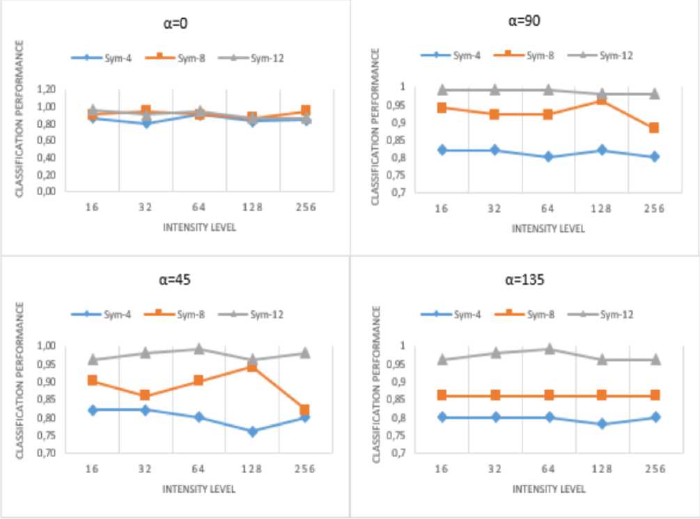
Fig.9. The classification performance (%) of DWT for different symlet values as the intensity level changes for different a values.

0.9

о

0.8

0.7

0.6

0.5

GLCM      GLTDM      Sym-12

16      32      64     128    256

INTENSITY LEVEL

Fig.10. Comparison of the classification performance (%) for GLCM, GLTDM, and DWT with sym-12 as the intensity level changes for а=135° .

• V.    Conclusion

This paper describes an alternative approach that utilizes Gray Level Total Displacement Matrix (GLTDM) which holds statistical information about the Discrete Wavelet Transform (DWT) of the original face image. The Haralick features are extracted from the generated four GLTDMs and a new feature vector is formed using these four groups of Haralick features to form JFV. Digital images usually require a very large number of bits and digital image compression is used to reduce redundancy of the image data required to store or transmit it over a communication link. Wavelets are mathematical functions and Symlet is one of the orthogonal wavelet families. The effect of changing wavelets, on the texture classification system performance and the application of wavelet transform to texture segmentation are the basic results of face recognition on wavelet decomposition structure. Symlet-4, 8, 12 tabs are used find out the best wavelet symlet for face recognition. Hence, it is finally concluded that DWT with sym-12 has superior performance than GLCM and pure GLTDM. Hence, face recognition shall have a new perspective on GLTDM technique and the classification performances will be improved if DWT with sym-12 is applied to the proposed GLTDM approach.