Дискриминантный анализ аминокислотного состава природных углеродистых веществ

The method of discriminant analysis of protein amino acid composition is widely used in biological, physiological, palaeontological and geochemical studies. For example, it allows to determine the taxonomic membership of the classes of shells of mollusk, brachiopods and bones of animals [11—13, 15], to identify intergroup differences in biological fluids and pathogenic minerals [1, 2], to determine affiliation to one of the microcommunities in hydrothermal systems [14].

Amino acids, found in sedimentary rocks, are not primary components of protein. They are in the bound state and included in the polymer components of organic matter or they form stable organic mineral complexes [3]. Amino acids are one of the most important indicators of the geochemical processes occurring in sediments. They characterize the degree of polymerization of fossil organic matter that is closely connected with the processes of postsedimentary deposit transformation. Heating effects contribute to both decay of amino acids, especially with a complex structure, and their formation due to the secondary synthesis.

Recently during our studies of amino acids in geological objects we accumulated material on the amino acid composition of different carbonaceous substances from asphaltites [8] to shungites [9]. Previously we made statistical evaluation of the similarity of the samples of shungites from various deposits by their amino acid composition and identification of the impact of shungite formation temperature on their amino acid composition [10].

The relevance of the studies of organic mineraloids is conditioned by debatable questions of their origin, the main of which is the problem of biogenesis or abiogenesis of initial substance, as well as the need of evaluation of physical and chemical conditions of formation.

The complex composition and structure hamper to study of natural solid bitumen and majority of other natural organic compounds. So we continued researches of the amino acid composition of solid bitumen by statistical analysis.

This work aims at the statistical estimation of differences in the amino acid composition of natural carbonaceous substances (CS) that a priori were separated into groups by physical and chemical features according to Uspenskys classification [6].

The objects of the researches were samples of natural solid bitumens from the carbonization sequence (asphaltites (albertite) — kerites (grahamite and impsonite) — anthraxolites), natural graphites, as well as samples of carbon black.

The tasks of the work were as follows:

• (1)    Establishing the most informative amino acids showing the greatest (statistically significant) differences between the groups of samples;

• (2)    Identification of statistically significant differences between groups of samples by several most informative amino acids simultaneously;

• (3)    Creation one or more of canonical discriminant functions (hereinafter - discriminant functions) based on these amino acids that best describe the differences in amino acid composition between CS groups and can be used for including new samples to one group or another.

Objects and methods

We selected 30 samples of natural carbonaceous substances, previously recognized and referred to certain types of organic mineraloids and minerals, as well as two samples of carbon black. The first and second groups included vein (samples 1—3) and clastic (samples 4—12) asphaltites from Timan-Pechora province and Eastern Siberia; the third (samples 13—15) — kerites from Timan-Pechora province; the fourth (samples 16—20) — the higher anthraxolites from Novaya Zemlya and Kazakhstan; the fifth (samples 21—27) — shungites of type I from Karelia; the sixth (samples 28—30) — coal graphite from Taimyr and Karelia, and the seventh (samples 31—32) — carbon black from Sosnogorsk Gas Processing Plant.

The identification and determination of amino acids in the samples were performed with the help of gas chromatograph GC-17A (Shimadzu, capillary column Chirasil-L-Val). The technique is described in [9].

The statistical analysis was carried out by the discriminant analysis (DA) in STATISTICA 6.0 program. The discriminant analysis of CS was conducted by the relative content of amino acids used as discriminant variables. The statistical evaluation was carried out for the level of significance p = 0.05.

Results and their discussion

At the first stage we checked the correctness of the initial division of samples into seven groups by thirteen amino acids (alanine (Ala), valine (Val), glycine (Gly), isoleucine (Ile), leucine (Leu), aspartic acid (Asp), glutamic acid (Glu), threonine (Tre), serine (Ser), phenylalanine (Phe), tyrosine (Tyr), proline (Pro), lysine (Lys)). On the basis of classification functions*, which are linear combinations of relative compositions of amino acids, it was determined that all the samples were initially classified correctly.

To identify informative amino acids, making the most significant contribution to the distinction between samples from different groups, we carried out DA by two methods: stepwise with inclusion; stepwise with exclusion [4]. As criteria of informative amino acid selection we used Wilks lambda statistics. The highest percentage of correct classification of samples (97 %) was obtained by stepwise with exclusion. Eight most informative amino acids — Ala, Asp, Tyr, Gly, Leu, Phe, Val, Ile was revealed by this method. The sets of samples from different groups differ statistically significantly by content of these amino acids. Six discriminant functions were calculated by these amino acids.

The number of discriminant functions, that significantly describe differences between the groups, was determined on the basis of their eigenvalues; relative percentage content of discriminant functions (i.e. percentage of explained dispersion); canonical correlation coefficient; and with the help of the test of significance of residual discriminantability of the system conducted using the Wilks lambda statistics and chi-square test (Table. 1, 2).

The value of eigenvalue and the relative percentage content are connected with discriminating abilities of the function: the larger they are, the greater is the discrimination. All discriminant functions do not necessarily provide a clear discrimination, but their positions are determined in accordance with their individual discriminant abilities. In our case, the first function with eigenvalue 10.6 provides the best discrimination, the second function (4.9) provides a maximal discrimination after the first function, etc. Similarly, if we consider relative percentage contents, it can be seen (Table 1) that the first function contains 51.87 % of the total discriminant abilities, the second — 23.99%, etc. For each subsequent function, this percentage decreases. The last functions are as weak, compared to the first ones, that they does not necessarily introduced a significant contribute to the definition of the differences between the groups.

The published results of DA showed that the feasibility of using discriminant functions for distinguishing objects can be best evaluated by the value of canonical correlation coefficient [4], which is a measure of the bond (the degree of dependence) between the groups and the discriminant function. If this coefficient is small, the discriminant function can be omitted for interpretation.

The coefficient of canonical correlation (Table 1) of the first four discriminant functions has values close to one; it is particularly high for the first two functions, which indicates to a strong dependence between the groups and the first two discriminant functions. The fifth and sixth functions possess relatively weaker relation with the groups. Based on the values of the canonical correlation coefficient, we can say that the groups are clearly different by the studied variables (i.e. relative contents Ala, Val, Gly, Ile, Leu, Asp, Phe, Tyr), otherwise all correlations could have small values. Evaluating relative percentage content and canonical correlations it is possible to determine how many and what discriminant functions are significant in determining differences between the groups.

Another criterion, to determine the number of discriminant functions, needed to determine differences between the groups, is to test the statistical significance of the residual discriminant ability of the system (discriminant functions) before calculating next discriminant function. Eight used discriminant variables are very effectively involved in distinguishing between the groups (Table 2). Wilks lambda close to zero (for k = 0) at significance level p < 0.05 indicates that there are significant differences between the groups yet before calculating of any of the discriminant functions. Therefore, it can be noted that the results have

Footnote:

The values and significance measures of discriminant functions (DF)

Таблица 1

Собственные значения и меры значимости дискриминантных функций (ДФ)

DF / ДФ	Eigenvalue Собственное значение	Relative percentage Относительное процентное содержание	Canonical correlation Каноническая корреляция
1	10.577	51.87	0.956
2	4.892	23.99	0.911
3	2.295	11.25	0.835
4	1.667	8.17	0.791
5	0.620	3.04	0.619
6	0.341	1.67	0.504

Table 2

Values of Wilks lambda statistics and chi-square test with subsequent excluded discriminant functions

Таблица 2

Значения статистики лямбда Уилкса и критерия Хи-квадрат с последующими исключёнными дискриминантными функциями

к	Wilks’ lambda Лямбда Уилкса	Chi-square Хи-квадрат	Degrees of freedom Степени свободы	p-level р-уровень
0	0.0008	168.541	48	0.000
1	0.009	110.990	35	0.000
2	0.052	69.310	24	0.000003
3	0.173	41.289	15	0.0003
4	0.460	18.237	8	0.020
5	0.746	6.901	3	0.075

Note. k — number of subsequently excluded discriminant functions beginning with one.

Примечание. k — коёичество посёедовaтеёь^о иcкёючё^^ыx диcкpими^a^т^ыx функций, ^aчи^aя с первой.

been obtained for the samples from the general set with differences between the groups. After excluding five discriminant functions (Table 2) the level of residual discriminant capacity is low (the value of Wilks lambda is close to one, the significance level p = 0.075). Consequently, the first five discriminant functions are statistically significant (as a whole as the system of functions). The remaining sixth discriminant function is statistically insignificant, so this function can be omitted.

Using the discriminant functions as a system, we can reduce the information, necessary for the discrimination of the groups, to the smallest number of dimensions, at which the significance of the discrimination is sufficient and the discrimination is correct. In the course of our analysis the dimension of the information space, needed to separate the samples into groups, decreased from original thirteen discriminant variables to eight most informative variables and further to five discriminant functions.

Now let us determine the relative contribution of individual discriminant variable in the value of each discriminant function. To do this the coefficients should be presented in a standard format (Table 3). The standardized coefficients are used to identify the variables that contribute to the value of the discriminant function. The larger the absolute value of the standardized coefficient of the variable, the greater the contribution of this variable to the value of the discriminant function.

The maximum contribution to the first discriminant function is made by the variables Ala and Gly, the following in significance contribution is introduced by Asp. All other variables are

Table 3

Standardized coefficients of discriminant functions

Таблица 3

Стандартизованные коэффициенты дискриминантных функций

Variable Переменная DF standardized coefficients / Стандартизованные коэ< )фициенты ДФ DF1 /ДФ1 DF2 / ДФ2 DF3 / ДФЗ ПР4/ДФ4 DF5 /ДФ5 DF6 / ДФ6 Ala -0.876 0.437 0.091 0.181 -0.221 -0.342 Vai -0.206 0.863 -0.452 0.283 0.329 -0.510 Gly -0.895 0.344 -0.115 -0.464 -0.080 0.134 He -0.081 1.084 -0.058 0.233 0.157 -0.286 Leu -0.335 -0.533 -0.680 -0.190 -0.394 -0.520 Asp -0.567 0.915 -0.544 -0.752 -0.427 0.055 Phe 0.120 0.497 0.749 0.309 -0.813 0.245 Tyr 0.00062 0.118 0.350 -0.735 0.206 -0.627 much less significant. For the second discriminant function three of the eight variables (Ile, Asp, Val) have relatively large standardized coefficients, so they introduce about the same contribution to its value. All other variables are compared to them are secondary. Phe, and Leu are dominant variables for the third discriminant function. But Ala and Ile, which contribute substantially to the first and second discriminant function, on the contrary, do not provide a meaningful contribution to the third discriminant function. Fourth discriminant function is marked by a great contribution of Asp, Tyr, and the fifth — Phe, all other variables are secondary importance.

To determine the closeness of the connection between the individual discriminant variables and discriminant functions, we will consider their correlation (its coefficients are termed complete structural coefficients). At a large absolute value of the coefficient all the information about the discriminant function is contained in the variable.

The first discriminant function (Table 4) is most closely associated with Ala and Gly, the second — with Val, Leu, Asp, the third — with Leu, Asp, Phe, Tyr, the fourth — with Asp, Tyr, the fifth — with Phe, Leu, Ile. Note that the discriminant functions 2, 3 and 4 do not have dominant (large) coefficients. At that the variables that contribute most to the values of the corresponding discriminant functions (Table 3) are generally most closely associated with these functions (Table 4).

Table 5 shows average values of the discriminant functions for each group of samples. Pairwise differences of these values for each function allow determining groups that are the best differentiated by this discriminant function. Figurative points on Figure 1 show geometrical arrangement of the samples rela- tively to each other at coordinate planes of some pairs of discriminant functions.

Table 5 shows that the discriminant function 1 discriminates mainly kerites and soot (Groups 3 and 7), as its average values for these groups are significantly different from each other and from the average values of other groups. Figure 1a shows that the samples of the seventh group are well differentiated from the samples of other six groups by the first discriminant function. The samples of the third group are different from the samples of other groups, although not as much as the seventh group of samples. The samples of other five groups do not differ so clearly by the first discriminant function. By discriminant function 2 samples of asphaltites (group 2) are significantly different from the samples of other groups, most strongly - from the samples of higher anthraxolites (group 4). The discriminant function 3 most strongly distinguishes kerites from higher anthraxolites (groups 3 and 4). Unlike the discriminant functions 1 and 2, it discriminates asphaltites from shungites (groups 1 and 5) (Fig. 1, b). It can be also used as auxiliary to the discriminant function 1 for separating kerites from shungites (groups 3 and 5). The discriminant function 4 well discriminates coal graphites (group 6) from other groups, especially from asphaltites (group 1), a bit worse from higher anthraxolites (group 4), well from shungites (group 5) (Fig. 1, c). It can be also used as auxiliary to the discriminant function 1 for discrimination of kerites from coal graphite (groups 3 and 6). The discriminant function 5 well discriminates asphaltites from kerites (groups 1 and 3) and can be used as auxiliary to discriminant function 1 for this discrimination. It also discriminates shungites from coal graphites (groups 5 and 6). Therefore, it can be used as auxiliary to discriminant function 4 for distinction of these groups.

Table 4

Complete structural coefficients

Таблица 4

Полные структурные коэффициенты

Variable Переменная	Complete correlations between disciminant variables and discriminant functions Полные корреляции между дискриминантными переменными и дискриминантными функциями
	DF1 / ДФ1	DF2 / ДФ2	DF3 / ДФЗ	DF4 / ДФ4	DF5 / ДФ5	DF6 / ДФ6
Ala	-0.944	-0.006	0.191	0.135	0.017	-0.112
Vai	0.442	0.533	-0.175	0.265	-0.111	-0.290
Gly	-0.883	-0.206	0.190	0.013	0.161	0.190
Не	0.176	0.316	-0.208	0.369	0.408	-0.075
Leu	0.142	-0.559	-0.466	0.185	-0.445	-0.419
Asp	0.375	0.548	-0.418	-0.505	-0.249	0.165
Phe	0.534	0.216	0.411	0.158	-0.636	-0.114
Туг	0.337	0.030	0.575	-0.576	0.060	-0.466

Table 5

Average values of discriminant functions for groups

Таблица 5

Средние значения дискриминантных функций по группам

Group No. Номер группы	Average values of discriminant functions / Средние значения дискриминантных функций
	DF1 / ДФ1	DF2 / ДФ2	DF3 / ДФЗ	DF4 / ДФ4	DF5 / ДФ5	ПР6/ДФ6
1	0.725	0.098	1.746	-1.634	1.228	-0.854
2	0.404	2.586	-0.792	-0.108	-0.395	-0.167
3	3.169	0.117	2.971	-0.172	-0.704	0.813
4	0.117	-3.075	-1.223	-1.389	-0.541	0.035
5	0.361	-0.318	-0.762	0.769	0.921	0.516
6	0.968	-2.164	0.593	2.559	-0.440	-0.849
7	-10.665	0.086	1.324	0.139	-0.221	0.193

Together five statistically significant discriminant functions well discriminate the seven groups of samples. Using these five discriminant functions allows unambiguously classifying new (previously ungrouped) samples.

In general, the informativeness of discriminant variables and efficiency of discriminant functions to interpret differences between groups are assessed by the percentage of correctly recognized (classified) samples. The classification* can be used with respect to the unknown objects to predict their affiliation to certain groups, and to verify the accuracy of the classification procedures in relation to the known objects [4]. The proportion of correctly classified objects testifies to the accuracy of classification* procedure.

The classification of the samples can be carried out by: classification functions, Mahalanobis distances squares, a posteriori probabilities of affiliation of samples to a group, which are calculated with the help of Mahalanobis distances squares.

The classification procedure uses discriminant variables themselves and/or discriminant functions. The classification procedure resulted in that only one sample (from the first group) was allocated to the other group (Table 6): a posteriori probability 0.49 for shungites (the fifth group), whereas for vein asphaltites (the first group) it is equal to 0.15. Although all other samples were classified by the program in accordance with the original partition into groups, low or not very high values of a a posteriori probability of some samples raise doubt in the correctness of the original classification, or point to individual physical-chemical or geological features of these samples. Thus, for sample 12 (clastic asphaltite, Eastern Siberia), a posteriori probability of affiliation to the given group 2 (clastic asphaltites) is 0.55, and to group 5 (shungites) — 0.42. A posteriori probabilities of affiliation to the given group of samples 16 (higher anthraxolite, Novaya Zemlya) from group 4 and sample 23 (shungite I, Nigozero) from group 5 are not high (0.65) compared to those for other samples from these groups.

Then we carried out classification with the help of five statistically significant discriminant functions. The obtained results were more accurate, because the impact of fluctuations was reduced [4]. It was established that all samples were correctly classified (Table 7). The results of the classification and the values of a posteriori probabilities of affiliation to a group, obtained by the discriminant functions and initial discriminant variables, were almost identical: the same samples (1, 12, 16, 23) had low or not very high values of a posteriori probabilities of affiliation to a predetermined group. Although the first sample was referred to the first group, but the probability of affiliation was low — 0.35.

Explanation of such results lies in the geological and geochemical characteristics of these samples. Sample 12 (Eastern Siberia), previously recognized as clastic asphaltite, was selected from a piece of bitumen with a heterogeneous phase content, which was a mixture of asphaltites and lower kerite and possibly higher kerite. This heterogeneity results in ambiguity of physical and chemical diagnostics of the sample and, accordingly, its affiliation to this or the other group of solid bitumen. Sample 16 (anthraxolite from Pavlovskoe deposit, Novaya Zemlya) is different from other anthraxolites samples (group 4) by the lowest degree of metamorphism [5]. If other anthraxo-

Footnote:

[ ф group 11 □ group 2 I ф group 3 | ▲ group 4 । • group 51 ■ group 6 I

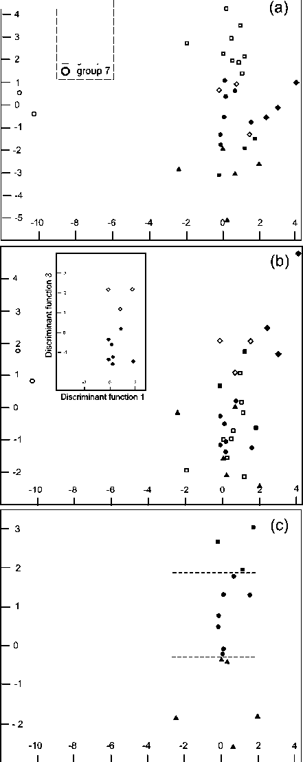
Discriminant function 1

Fig. 1. Location of samples in the planes defined by the discriminant function 1 and 2 (a), 1 and 3 (b), 1 and 4 (c). Inset (b) shows the location of the samples of groups 1 and 5. Figure (c) shows the arrangement of samples only for groups 4, 5 and 6. The dashed line separates groups for discriminant function 4

Ðèñ. 1. Ðàñïîëîæåíèå îáðàçöîâ íà ïëîñêîñòÿõ, çàäàâàåìûõ äèñ-êðèìèíàíòíûìè ôóíêöèÿìè 1 è 2 (à), 1 è 3 (b), 1 è 4 (c). Íà âðåçêå (b) ïîêàçàíî ðàñïîëîæåíèå îáðàçöîâ ãðóïï 1 è 5. Íà ðèñ. (c) ïðèâåäåíî ðàñïîëîæåíèå îáðàçöîâ òîëüêî äëÿ ãðóïï 4, 5 è 6. Ïóíêòèðíûå ëèíèè ðàçäåëÿþò ãðóïïû ïî äèñêðèìèíàíòíîé ôóíêöèè 4

Classification of samples by means of a posteriori probability

Классификация образцов с помощью апостериорных вероятностей

Таблица 6

Sample No. Номер образца	A posteriori probabilities / Апостериорные вероятности
	Group Группа	1 р‘= 0.094	2 р = 0.281	3 р - 0.094	4 р = 0.156	5 р = 0.219	6 р - 0.094	7 р = 0.063
X"	1	0.145902	0.342200	0.026250	0.000044	0.485377	0.000227	0.000000
2	1	0.999940	0.000016	0.000000	0.000000	0.000044	0.000000	0.000000
3	1	0.998936	0.000001	0.000701	0.000321	0.000040	0.000001	0.000000
4	2	0.000008	0.995053	0.000000	0.000000	0.004939	0.000000	0.000000
5	2	0.000008	0.997457	0.000000	0.000000	0.002534	0.000001	0.000000
6	2	0.003769	0.880480	0.000205	0.000008	0.115497	0.000040	0.000000
7	2	0.000000	0.999999	0.000000	0.000000	0.000001	0.000000	0.000000
8	2	0.000000	0.999945	0.000006	0.000000	0.000049	0.000000	0.000000
9	2	0.000541	0.999393	0.000000	0.000000	0.000066	0.000000	0.000000
10	2	0.000066	0.956917	0.000008	0.000001	0.043008	0.000000	0.000000
11	2	0.000015	0.972746	0.000000	0.000000	0.027239	0.000000	0.000000
12	2	0.025804	0.552375	0.002468	0.000000	0.419180	0.000172	0.000000
13	3	0.003209	0.000257	0.993735	0.000004	0.002218	0.000577	0.000000
14	3	0.000007	0.000000	0.999993	0.000000	0.000000	0.000000	0.000000
15	3	0.001303	0.000005	0.997811	0.000001	0.000861	0.000020	0.000000
16	4	0.000036	0.000107	0.000000	0.652913	0.346483	0.000461	0.000000
17	4	0.000005	0.000001	0.000000	0.994323	0.005670	0.000001	0.000000
18	4	0.001424	0.000000	0.000001	0.998015	0.000558	0.000002	0.000000
19	4	0.000000	0.000000	0.000000	0.999775	0.000002	0.000223	0.000000
20	4	0.000008	0.000000	0.000000	0.999882	0.000108	0.000002	0.000000
21	5	0.000052	0.000801	0.000002	0.000366	0.992301	0.006479	0.000000
22	5	0.000760	0.003653	0.000010	0.005140	0.990370	0.000067	0.000000
23	5	0.001392	0.347572	0.000000	0.000044	0.650987	0.000005	0.000000
24	5	0.001948	0.007585	0.000007	0.000000	0.988826	0.001633	0.000000
25	5	0.000103	0.066369	0.000000	0.000073	0.931659	0.001796	0.000000
26	5	0.000103	0.000653	0.000000	0.040185	0.955941	0.003117	0.000000
27	5	0.000209	0.000045	0.000001	0.012673	0.980705	0.006367	0.000000
28	6	0.000000	0.000007	0.000001	0.000014	0.037823	0.962154	0.000000
29	6	0.000000	0.000000	0.000000	0.000262	0.000696	0.999042	0.000000
30	6	0.000329	0.000000	0.000141	0.000017	0.003156	0.996356	0.000000
31	7	0.000000	0.000000	0.000000	0.000000	0.000000	0.000000	1.000000
32	7	0.000000	0.000000	0.000000	0.000000	0.000000	0.000000	1.000000

Notes. *p — a posteriori probabilities of affiliation of samples to groups, proportional to size of groups, ** — incorrect classifications

Примечания. *p — априорные вероятности принадлежности образцов к группам, пpoпopциo^aль^ыe размерам групп, — íåïðàâèëüíûå êëàññèôèêàöèè.

lites from this group belong to the class of higher anthraxolites, then this sample is closer to the average anthraxolites. Sample 23 (shungite I from Nigozero), in contrast to the primary migration shungites (samples 21, 22, 24—27), refers to redeposited shungites, which organic matter was buried as clots in coastal shallow water zone, and then during tectonic processes transferred as part of tuffaceous detrital materials [7]. This resulted in significantly greater contamination by mineral impurities of this shungite compared to others.

Conclusion

• 1.    The dimension of the information space, needed to discriminate samples into groups, by the multivariate statistical analysis, decreased from original thirteen discriminant variables (amino acids) to eight (the most informative discriminant variables) and then to five discriminant functions, the number

• 2.    Using standardized coefficients and complete structural coefficients we determined the most significant discriminant variables (no more than three amino acids) for each discriminant function. Herewith the set of discriminant variables is individual for each discriminant function. Each of them allows significantly discriminating two or more groups of natural carbonaceous substances.

• 3.    The results of the classification and values of a posteriori probabilities of group membership, obtained by canonical discriminant functions and initial discriminant variables, are similar. Further statistically significant discriminant functions can be used for a more accurate (compared to discriminant variables) grouping of new (previously ungrouped)

• 4.    The multivariate statistical analysis of amino acid composition of natural hydrocarbons can find samples, wrongly related to other group as a result of unreliable physical and chemical diagnostics, and also determines samples different from the samples of their group by geological and geochemical characteristics. This indicates the possibility of applying such an analysis for comparative grouping of natural hydrocarbons.

of which was established with the help of such characteristics as canonical correlation coefficient, test of significance of residual discriminant capacity of system.

Classification of samples by a posteriori probability in the space of two statistically significant discriminant functions

Òàáëèöà 7

Классификация образцов по апостериорным вероятностям в пространстве пяти статистически значимых дискриминантных функций

Sample No. Номер образца A posteriori probabilities / Апостериорные вероятности Group Группа 1 р = 0.094 2 р = 0.281 3 р = 0.094 4 р = 0.156 5 р = 0.219 6 р = 0.094 7 р = 0.063 1 1 0.348381 0.330691 0.015794 0.000035 0.304561 0.000537 0.000000 2 1 0.999455 0.000044 0.000006 0.000000 0.000495 0.000000 0.000000 3 1 0.991720 0.000002 0.007266 0.000789 0.000223 0.000001 0.000000 4 2 0.000007 0.991756 0.000000 0.000000 0.008236 0.000000 0.000000 5 2 0.000007 0.995271 0.000000 0.000000 0.004722 0.000000 0.000000 6 2 0.005058 0.862462 0.000290 0.000008 0.132128 0.000054 0.000000 7 2 0.000000 0.999998 0.000000 0.000000 0.000002 0.000000 0.000000 8 2 0.000000 0.999930 0.000009 0.000000 0.000060 0.000000 0.000000 9 2 0.000529 0.999362 0.000000 0.000000 0.000108 0.000000 0.000000 10 2 0.000269 0.981763 0.000003 0.000001 0.017964 0.000001 0.000000 11 2 0.000013 0.951049 0.000000 0.000000 0.048939 0.000000 0.000000 12 2 0.046447 0.563077 0.002530 0.000000 0.387638 0.000308 0.000000 13 3 0.006054 0.000267 0.990572 0.000004 0.002021 0.001083 0.000000 14 3 0.000006 0.000000 0.999994 0.000000 0.000000 0.000000 0.000000 15 3 0.052178 0.000029 0.945718 0.000005 0.001296 0.000775 0.000000 16 4 0.000140 0.000148 0.000000 0.726777 0.271146 0.001790 0.000000 17 4 0.000016 0.000001 0.000000 0.995736 0.004243 0.000004 0.000000 18 4 0.003027 0.000000 0.000001 0.996453 0.000515 0.000004 0.000000 19 4 0.000000 0.000000 0.000000 0.999955 0.000007 0.000038 0.000000 20 4 0.000014 0.000000 0.000000 0.999874 0.000108 0.000003 0.000000 21 5 0.000090 0.000831 0.000002 0.000357 0.987555 0.011165 0.000000 22 5 0.012203 0.011381 0.000007 0.010817 0.9645 35 0.001058 0.000000 23 5 0.001755 0.315878 0.000000 0.000040 0.682321 0.000006 0.000000 24 5 0.002125 0.006266 0.000009 0.000000 0.989825 0.001774 0.000000 25 5 0.000109 0.054388 0.000000 0.000060 0.943544 0.001898 0.000000 26 5 0.000285 0.000853 0.000000 0.046006 0.944303 0.008552 0.000000 27 5 0.001306 0.000086 0.000001 0.018939 0.940391 0.039277 0.000000 28 6 0.000000 0.000008 0.000003 0.000019 0.080956 0.919014 0.000000 29 6 0.000000 0.000000 0.000000 0.000218 0.000731 0.999050 0.000000 30 6 0.000321 0.000001 0.001873 0.000049 0.021526 0.976231 0.000000 31 7 0.000000 0.000000 0.000000 0.000000 0.000000 0.000000 1.000000 32 7 0.000000 0.000000 0.000000 0.000000 0.000000 0.000000 1.000000 samples, because their use reduces influence of random fluctuations.

The researches were carried out with the partial support of the Program of Fundamental Researches, UB RAS No. 15-18-55, the amino acid composition was determined by analytical equipment of CCU Geoscience Institute of geology KomiSC UB RAS.