Дрейфово-компрессионные волны, распространяющиеся в направлении дрейфа энергичных электронов в магнитосфере

Magnetospheric plasma exhibits a wide spectrum of ultralow-frequency (ULF) oscillations, also called geomagnetic pulsations. They are identified with magnetohydrodynamic (MHD) waves. From both observational and theoretical viewpoints, they can be divided into two large groups: waves with small values of azimuthal wave number m and waves with large values of m [Yeoman et al., 1992; Leonovich, Mazur, 1993; Fenrich et al., 1995].

Waves with small m values have predominantly toroidal polarization, i.e. the wave magnetic field lines oscillate in the azimuthal direction. They have large azimuthal dimensions and can be observed with groundbased magnetometers. They are sometimes called transverse large-scale oscillations. Usually these waves are identified with Alfvén modes whose sources are located in the outer magnetosphere. A fast magnetosonic (FMS) wave, originated from the magnetopause or the solar wind, is assumed to propagate into the inner magnetosphere, where it generates an Alfvén mode in the field line resonance, at which the FMS wave frequency coincides with the local eigenfrequency of the field line resonance [Chen, Hasegawa, 1974; Southwood, 1974].

Waves with large values of the azimuthal wave number have largely poloidal polarization, i.e. the wave magnetic field lines oscillate in the radial direction. They have small azimuthal dimensions and represent more local events than oscillations with small m. These waves can be called transversely small-scale. They are usually identified with poloidal Alfvén modes. The waves are believed to arise from processes occurring in the inner magnetosphere. Due to ionospheric shielding, geomagnetic pulsations with large azimuthal wave numbers can be experimentally studied only with the aid of artificial Earth satellites or radars.

Among the waves with large m in the Pc5 range there is a group of storm-time compressional oscillations whose frequencies can be much lower than the fundamental frequency of Alfvén resonance in the given L shell. Such oscillations can be recorded both by satellites [Barfield, McPherron, 1972] and by groundbased radars [Allan et al., 1982].

There is still no consensus on the physical nature of the storm-time compressional Pc5 pulsations. According to the magnetohydrodynamic theory, this should be the lowest-frequency mode – the slow magnetosonic mode. However, it is not entirely clear whether the MHD approximation is valid for describing oscillations with frequencies much lower than the Alfvén range in a collisionless plasma since in this case bounce frequencies should be taken into account, which can correctly be done only with the kinetic approach [Hurricane et al., 1994 ]. Storm-time Pc5 pulsations are sometimes associated with drift mirror modes, which are kinetic in nature [Kremser et al., 1981, Pokhotelov et al., 2001]. Still, satisfying mirror instability conditions requires strong temperature anisotropy in magnetospheric plasma.

In our opinion, drift-compressional modes are best suited for interpreting most storm-time compressional Pc5 pulsations. They are the most common compressional modes in kinetics since they demand for their existence only finite plasma pressure and inhomogeneity across magnetic shells. In this case, the instability of the drift-compressional modes can arise from spatial gradients of hot plasma density [Crabtree et al., 2003; Klimushkin, Mager, 2011], inverted distribution of hot proton energy [Mager et al., 2013], or from the coupling with the Alfvén mode due to magnetic field line curvature [Klimushkin et al., 2012]. By the inverted distribution is meant the nonmonotonic velocity distribution with its maximum in the high-energy part of spectrum, by analogy with [Hughes et al., 1978]. A characteristic feature of drift-compressional waves is the dependence of their frequency on the azimuthal wave number. A similar behavior pattern has been found in radar data [Mager et al., 2015; Chelpanov et al., 2016].

It has been shown that the drift-compressional modes propagating in the direction of the drift of high-energy protons interact resonantly with them. As temperature increases and particle density decreases with distance away from Earth, this can cause instability and a spontaneous increase in waves whose phase velocity direction coincides with the proton drift direction [Mager et al., 2013]. The instability threshold is lowered if the proton distribution function is inverted. However, as shown in [James et al., 2013], in some cases there are waves propagating in the opposite direction, i.e. in the electron drift direction. Therefore, in this paper we study the situation in which the wave propagates in the electron drift direction. Here, we assume that there are hot protons and electrons in plasma, the latter having an inverted energy distribution.

MODEL OF ENVIRONMENT AND BASIC EQUATIONS

We use an axially symmetric model of the magnetosphere, which takes into account the field line curvature and the background plasma inhomogeneity across magnetic shells and along field lines. To do this, we introduce an orthogonal coordinate system { x ¹, x ², x ³} such that the coordinate x ¹ coincides with the magnetic shells, x ² indicates a magnetic field line (azimuthal coordinate), and x ³ is a field line point; g 1 , g ₂, and g ₃ are respective coordinates of a metric tensor; dl = ^ g 3 dx ³ is the length element along the field line [Leonovich, Mazur, 1989]. Taking into account the curvature and field-aligned inhomogeneity of the magnetic field makes particles trapped in the magnetosphere.

We consider plasma with an admixture of hot protons and electrons. Since the contribution of cold particles to the total plasma pressure is small, we consider only the contribution of hot particles. Here we assume that the protons have a Maxwell energy distribution:

n p

F p =------T exP

(2nS)2

and the hot electrons have an inverted distribution and are modeled by the following function:

Here, n p and n e are proton and electron densities respectively; ε= v ²/2 is the mass-normalized particle energy; V is the particle velocity; S is the positive integer; G (...) is the gamma function; £₀ and £₀ are pe the parameters proportional to the squared thermal velocity of particles. Hereafter, the indices “p” and “e” are the proton and electron variables respectively.

Note that with S =0, electron distribution function (2) becomes the Maxwell distribution. For S >0, electrons have the mean particle energy £ _e = ( S + 3/ 2 ) e ₀ e and energy at maximum £ = S £_n .

^e max         ⁰ e

We employ the axially symmetric model of the magnetosphere. The dependence of disturbed parameters on time and coordinates is represented as exp [- i re t + i J k1 (x1) dx1 + ik 2 x2 J, where ω is the wave frequency; k1 and k2 are the radial and azimuthal wave vector components respectively.

Plasma oscillations with a frequency less than the gyrofrequency of plasma particles can be considered within a gyrokinetic framework in the WKB approximation [Chen, Hasegawa, 1991]. In the approximation in which the wave frequency is much less than the bounce frequency of particles, an equation describing the drift-compressional mode can be derived from the gyrokinetic equations presented in [Chen, Hasegawa, 1991]. However, unlike previous works [Crabtree et al., 2003, Klimushkin, Mager, 2011; Mager et al., 2013] which took a wave whose direction of propagation coincided with the proton direction k ₂<0, i.e. to the west, we consider the case where the wave propagates east, in the electron drift direction k 2 >0.

Thus, we study the electron wave–particle resonance: in the equation for the drift-compressional mode, the sign in the resonant denominator of the term describing the contribution of hot protons changes to positive, i.e. no wave-particle resonance exists for protons, but it exists for electrons, and the sign in their resonant denominator becomes negative:

b ( i ) = 4 ⁿ m p

p ( p b | ( l )) U

Here b || is the longitudinal component of the wave magnetic field; l is the distance along the field line from the magnetic equator to a given point; ... is the velocity space integral:

+^

- to

e

X

—11

S

*

to,

";

. 5+2 S

e

e

- "2

e

X

*

= 4nf (...)^d ц d е; uJ

(...) is the average over the bounce period τb:

(...) = 7J- °₀(^luj ^{dl ; T} = ² J - °₀KI ^d1 , i _b 0 0

where ± l 0 denotes the reflection points on the ionosphere for particles with energy ε and magnetic moment ц = u ² /(2 B ); m _p and m e are the proton and electron masses respectively; to _d p e is the drift frequency:

tod = klV^d dp,e     | x dp, e

k ₂     ( 1 B '

® c_oe4g I 7 g 1 ² B p, e

R

where v and v _B are the longitudinal and transverse particle velocities; V _d is the particle magnetic drift velocity; to c p e = eB / m _p , _e is the gyrofrequency; R is the magnetic field curvature radius. The operator Q ^ˆ is determined as follows:

d

Qpe = to;i~± ' de

k2      1 d tocp,e Vg2 givdx1

Here, the sign “+” indicates protons; the sign “–” marks electrons.

After changing variables s, p^c, X such that X =sin² a =p B ₀/s, a is the pitch angle, B ₀ is the magnetic field at the equator, " = ^e / e ₀, equation (3) can be represented as

B 0

B ( 1 )        1 0 ( X )

b ( 1 ) = J d X J dl

, B ( 1 ) X ² Л ( to , X )

B ₀ u ( 1 , X ) u ( 1 ‘ , X )

b ( 1 ‘ ),

where

u ( I , X ) = 71 -X B ( I )/ B ₀,

во

Л ( to , X ) = —p L b _p

, Z 3 ^в0₌

I (to, X) + p        2 Lbe Г(S + 5/2)

П

I e ( to X ),

+to

" p e " 2

—;—----X

"2+® / n

X

®np _ toQd  Q dpdp

*

A tor

E2 1^

"p +2

y^ d p

,

Q de

" 2

to ee

The variables

*

to„ np

*

to„ ne

and

*

toE ep

*

to ee

Q de

Q,

d e

1	a- 2 e 0	n p
g 1	to c p T g T	, n p
1	k 2 e 0	n e
g	1 to c e T g	2 n e
1	k 2 e 0	e‘ 0p
g 1	toc v g r c p 2	e 0 e
1	2 e 0	e‘ 0 e

e g 2 e0e

g1 to

correspond to

—►

*

the diamagnetic frequencies to'

— —

= k _± V * ,

where V ^* is the velocity of the particle diamagnetic drift driven by the radial gradient of plasma density or temperature; Q _d = to _d e ₀ / e is the bounce-period-averaged drift frequency of particles with energy ε 0 ;

p ₀ is the parameter describing the ratio of plasma pressure to magnetic pressure at the equator; L b is the particle path length for the bounce period:

L b = u T _b = 4 J 0 ⁰ u ( I , X ) ^{- 1} d1 .

In the dipole magnetic field, L _b and Q _d weakly depend on X : L b - 1.3 - 0.56VX and Q _d - 0.35 + 0.15VX [Hamlit et al., 1961]. Therefore, we assume that Л is independent of X . Then, in Equation (4) we can take Л outside the integrals. Next, we can carry out a number of transformations, as in [Mager et al., 2013], and obtain a second-kind homogeneous Fredholm integral equation with a symmetric kernel. This equation can be solved numerically. In this case, we get sets of eigenfunctions b_N and eigenvalues Л N in the integral equation, which determine the field-aligned structure and eigenfrequencies of drift-compressional modes. As shown in [Mager et al., 2013], drift-compressional modes are localized(5i)n the vicinity of the geomagnetic equator. This agrees with satellite data on compressional Pc5 pulsations [Higuchi, Kokubun, 1988].

EIGENFREQUENCIES

AND INSTABILITY CONDITIONS

The eigenfrequencies are determined from the dispersion relation Λ (ω)=Λ _N , i.e.

_ ^P0 p           3 Pl

Лд, =   I „ ( to ) +

N L b _p^p"' 2 L b e Г ( 5 + 5/2)

0 e

п

I М

p

After taking the integrals, we have

^Л n =

P p

3 в,

Here

L b p

f ( ю ) + -^p2 L b

e

(О ю f,(ю) = -Ю 1 — ^e-

Q,

d e

Q,

'de J

to

ю

^f _; ^{( ю ).}

Now, to find the eigenfrequencies and possible instability increments, we represent the wave frequency as ω=ω 0 + i γ. We consider the real part of frequency as being much larger than the imaginary part: ю ₀ » y .

Suppose a = Qd / Qd , then, by changing variables ep in Expression (8), we can rewrite the dispersion relation as

-

• ю. ю

V

Q de

•

Q_d d e J

+

L bp_ Л = f

P p N ^Л

3 P e

2 P p

/    3

ю

()

V ^d e J

Q de

Q de

)

*

ю

1 — / e

Qd de

п

X

Г ( 5 + 5/2 )

+

( A ю

Qd , de

•              • ю ne . 3 ЮЕе

Q de

2Q de

x

Z C

п

to

x 5 + 1 - m

Qd , de

+

The parameter a represents the ratio of electron energy to proton energy: a = m £0 / m £0 . For epp simplicity, we take hot proton and electron densities, which contribute to plasma pressure, as being equal. Then, a can be represented as

m = 0

5 + 3

Z

,

a = 3 ^{в 1}

2 P p ( 5 + 3/2)

.

where Z

is the

plasma dispersion function

[Walker, 2005],

Z

^f р^{( ю )} =

+to

e - 1 ²

dt .

+

- to t

e

•

ю

_ ^Lp +

8 Q_d d_p

*              *

ю„    з ЮЕ n p          4

•

Ю ^Ю Е _Р Ю

^^^^^^B  ^^^^^^^^^^^^^^^^^^^^^^^B  ^^^^^^B

Qd,

2 Q d,

Qd,

Qd Qd dpd

x

(

x

Ю

^^^^^^B

^^^^^^B

Qd,

1 ю --+

(

ю e—12

where function:

Z ⁺

, e - t dt.

2 Q

Z ⁺

,

t2 + ю / Qa dp

-dt =

is the complementary error

If we consider the case close to the ring current conditions, then we can say that the proton energy is much higher than the electron energy, i.e. a ^ 1 and, accordingly, P _e / P _p ^ 1. Then, we can expand the function f _p ( aю / Q d e ) of Expression (11) in the small parameter a . Neglecting all terms such that the power of a is greater than 1, we get

л

A

•

ю fn a--- p I Qd , de

3 ^ю E,

4 Pd.

^^^^^^B

a

ю

ю,

*

n

^ю n

Qd,

^^^^^^B

Qd de

V

Q_d d p J

.

To find an analytical solution, we expand f , ( ю / Q d e ) in the small parameter for two extreme cases: when the eigenfrequency is much less than ( ю / Q d e ^ 1 ) and much greater than ( ю / Q d e » 1 ) of the electron drift frequency.

EIGENFREQUENCY MUCH LESS THAN ELECTRON DRIFT FREQUENCY: ω/Ω =1 d _e

If we expand Z (^ ю / Q d e ) in the small parameter ю / Q _d e ^ 1 in f . ( ю / Q _d e ) and neglect all terms where the power of ю / Q _d e is 2 or more, considering them small, we derive the expression

*     ^* ,     to            to .       to .          to / --- =--L + —s_ +--- e Qd       Qd   Qd    Qd V d e 7 V d e        d e 7       d e	<       • A 3 to d e 2 Qd d e
	S + 3 2 V         7

velocity is lower than the mean particle magnetic drift velocity in the bump in the inverted distribution.

The wave existence conditions for to / Q_d ^ 1 from d _e

(14) are as follows:

Then, for the case when the wave eigenfrequency is much less than the electron magnetic drift frequency, and the proton energy is much greater than the electron energy, the dispersion relation takes the form

Le л Pp N = 3 = 4 toE + Qd V dp • A to np 1 2 to a. Qd de ( 3 2 V to + ^p. Qd dp 7 - Qd dp 7 - 3 . Г to * - + toe. Qd ede A Й ( 3 -ton 2 ^ e (13) 2 Pp VQd 7 Qd de V S + 3 2 7 . or

[	* 3 to		* to 1 n
		e		— >  0,
	4 Q d		2 Qa d
< L b A	3	e * toE toe+	* to n p	p + 3 ■	* toe	* to +-to	(16.1) > 0
A N	4	Qd V d p	Q d p 7	2 P p	V Q d e	Q d e 7

	3 4 *		* to n e _ — Q d e *	* 1 to n. p- <  0,
				2 Q d p A		**	(16.2)
, toe Л	3	to£ £ p	to + - n p-		+ 3 Be	to      to E e + n e	< 0.
Л N	4	V Q d p	Q d p	7	2 P p	Qd   Qd V d e         d e 7

From (13), we derive the eigenfrequency expression:       The instability γ> 0 takes place for (16.1) with

to = Q dp x
L b	to=„      to n	3 e e	to £      to n
—p-A	—p_ + —p_
P p N 4	Qd   Qd V d p        d p 7	2 P p	V Q de Q de
x		*
	3 to n e	1 to n p
	4 Q de	2 Qd dp

	Cto. A	A      * A toE	to„        toE
	0 - S 1	1 '	ne- +-- ' <  0         (17.1)
	Qd      j d e	Qd d e	Qd 2 Qd d e d e
and for (16.2) with
	On	toE	to„        toE
	0 - S	1^	--n^ +-- ' <  0        (17.2)
	Qd j d e	Qd d e	Qd 2 Qd d e d e

To find the increment, we calculate the imaginary part of dispersion relation (11), apply the expansion in the small parameter to the plasma dispersion function, and neglect the terms in the denominator, where the power of to / Q d e is 2 and more:

In the equatorial parabolic approximation for the dipole magnetic field for the first harmonic N=1, we can take that A. ® 0.5/ L and L = 2nV2L, where L is 1                                    bp, e the distance to the magnetic shell in the equatorial plane [Mager et al., 2013]. Then

Y = -Qd6

e

Г (S + 3/2)

	C        A toL - s VQ d e 7	* 1 - tofe. Qd d e	-to^+ 3 to, Q d e 2 Q d e _	. (15)
* 3 to n e 1 to n p

4 Qd 2 Qd ded

to.. = n p	k 2 8 0 p n p to„ L n c p p	, to£ b p	k 2 e0 e° 20 p 0 p
				to„ L en c p 0 p
	3 k 2to	*		k 2 ^ 0 n e
Qd dp
	toc L 2			,
		n e		tor L n
	c p			c e      e              (18)
* tor	= - k 2 4	so 0e	Q	3 k 2 E 0e d e 2 . to L c e
εe	tor L c e	£ 0 e

From eigenfrequency expression (14) it follows that the wave can exist in plasma without particle temperature and density gradients. Equations (14) and (15) also show that without these gradients the instability occurs only for the inverted distribution ( S ^ 0). In this case, to / Q d e - S <  0, then V_ph <  V d ( ^s = ^s e_max ) . Hence, in the absence of plasma gradients the instability can occur if the wave phase

Wave conditions (16) for the first harmonic in the parabolic approximation for the magnetic field can be written as

<

^L P p

9 и	' n p
— + 2 -	e- —p:	> 0,
2 Ln	e n p
f!L + n p.	- 2 B e	£0e n 0 e । e
= 0 p n p ,	P p	to n e

(19.1)

1

^L Р р

9      п'

— + 2 -e -2Ln e

n _p

^£ 0р ⁿ р 7

^^^^^^в

П ‘

n p

2 ь [fse.+i

(19.2)

L bp- Л P p

- 3 b«£ N = 4 Q

*

1 £

^m -

-

id    Qd dpd

1 m a

2 Qd de

*

3. «

2 Q,

V

' dp J

.

^Р Р (^е<

0 n e e

Instability condition (17) in this approximation is for

(19.1)

«0. kd de

- 5

3 ^е0, — + —

L

V

Ч

- ‘

+ — n _e

^^^^^^в

3 £‘

3 0 <  0

^{2 £} 0 _e

(20.1)

3 P e

m

2 Р р «,

de

m

1--£

Qd de

V

* ^m £e ^Q de

^M - e ₇

^Q de J.

From (21) we derive the eigenfrequency expression: ^m 0 = ^Q d_p ^X

and for (19.2)

L bp Λ

P p N

X-------

*

1 £

3 ^m

4 Q,

^m n.

Q dpd

+ ^{3 P e}

2 Р р V

* m£e Qd de

« 0

Qd de

^^^^^^в

Г

I 3

5 - +-e-

£0,

Л

L £0

V ⁰ e 7

£

+ n e - ³⁰ >  0.

n e    ^{2 £} 0 e

(20.2)

^^^^^^^_  ^^^^^^B

*

mE^ I 5 + 3

Q de

^^^^^^B

*

1 ^m n p

m„

_2e_

Qd de J

.

2 J 2 Q_d d_p

Thus, waves with frequencies much less than the electron magnetic drift frequency can propagate in the electron drift direction if condition (19.1) or (19.2) holds. This is possible even in the absence of plasma temperature or density gradients, i.e. only due to magnetic field inhomogeneity. At the same time, these waves can growth if the electron temperature and density gradients correspond to condition (20.1) for (19.1) and to (20.2) for (19.2).

The instability can exist for the Maxwell distribution of electron energy due to the temperature and density gradients 5=0. nе / ne * 0, £0e / £0e * 0. Without these gradients, the instability can be caused by the inverted distribution of electron energy     5 * 0, nе / ne = 0, £0=/£0e = 0),  nP / np = 0,  e0 / £0  = 0. The ee        pp greatest increase in the wave occurs with multidirectional radial gradients of electron temperature and density.

To find the increment, we again use the expansion in

the small parameter and neglect

denominator,

where the power

of

the terms in the

Q / m is 2 and d _e

more:

Y = -Qd.

X

П

X 5 +5/2     m₀

« 0 ' _p ^d?

Qd I de

1 e    Г (5 + 3/2)

_«_l - 5

V^Q de .

mr

1£^

Qd de 7

*

3 ^m £e

^^^^^^^B  ^^^^^^B  ^^^^^^^^^^^^^^^^^^^^B

4 Qd de

^^^^^^B

X

* ^m n e

Qd de

+ -

*

mE

^£ e

^^^^^^B

2 Qd de

*

1 « - p,

2 Qd dp

.

Expression (22) shows that the wave, as for m / Q_d ^ 1, can exist in the absence of the gradients. e

For the wave to exist, the following conditions should hold

EIGENFREQUENCY FAR

EXCEEDING ELECTRON DRIFT

FREQUENCY: о/Q » 1

d _e

If we expand Z (^m / Qde) in the small parameter Qde / m ^ 1 in f. (m / Qde) and neglect all terms such that the power of Qd / m is 2 or more, considering e them small, we obtain the expression

Lb^ Л к

or

N

^^^^^B

*

3 ^m £ e

^^^^^^^B  ^^^^^B  ^^^^^^^^^^^^^^^B

4 Q de

3 m

*

)

^£ p

4 Q

p

e

Q„ dp 7

*

3 ) - 1 ^ n t- >  0.

2 7 2 Q _dp

3 Р

2 Р,

e

p

**

m m

-^£^ + - ⁿ^ > 0

Q, Q de

e

(24.1)

	m	m	r	« £ e	« £   m -
f e			1 -			—- + —-
	d e	Qd d e	V	Q d e		Qd  Qd V d e        d e 7

1

*

3   ^m £ e

^^^^^^^B  ^^^^^B  ^^^^^^^^^^^^^^^^^^B

^{4  Q} d e

^^^^^B

2 7 2 Q _d

*

m

< 0,

L _b p Λ

^P p

N

^^^^^B

**

3 m   m

3     ^£ p +__ 2 p_

4 Qa   Qa

V ^dp ^dp J

3 Р

2 P,

e

p

*

)

£

e

*

)

n _e

e

Q. Q de

< 0.

(24.2)

Thus, in the case when the wave eigenfrequency is much greater than the electron drift frequency and the proton energy is much greater than the electron energy, the dispersion relation is expressed as:

The instability condition from (23) for (24.1) is

.«l - 5

^Q d e

1 Q„

m -.    3 m £

Qde 2 Qd= ee

(25.1);

and for (24.2),

-m0- - s

^Q d e

ЮЕ

1--~

Q

^m n e + 3 ^m

n 2Q ee

(25.2)

In the parabolic approximation of magnetic field for

the first harmonic N =1, the wave existence can be written as

conditions

<

or

<

3 Г s+31+^ Г s+3

L

L B p

⁴ 7 ^p 0_e

n _p

S np 7

¹ ~ >  0, 2 n p

2 Be P0e + nL в (p0e ne 7

3 Г s + 3      Г s + 3

L

⁴ 7 ^p 0_e

¹ n <  0, 2 n p

n _p

(26.1)

L в р

^e 0 p ⁿ p 7

(26.2)

в (р.

^; 0e n e J

The instability condition for (26.1) is

Г ^m 0

Qd de

е' ^

s 3 +   +

L

(

еп

0 e 7

and for (26.2),

Г «0.

I Qd de

- s

е.

—+—-

0 e

L p0(       0e 7

p'

ⁿ e - ³⁰ <  0

n e ^{2 p} 0 _e

(27.1);

n '

+ — n _e

3 е'

3 0 >  0.

2 е0

0 _e

(27.2)

Waves with frequencies much electron magnetic drift frequency when the proton temperature and

greater

than the

m / Qd > 1 exist de density gradients

satisfy condition (26.1) or (26.2). As for m / Qd ^ 1, e the wave can exist in the absence of such gradients. The instability develops if the electron temperature and density gradients meet condition (27.1) for (26.1) and (27.2) for (26.2).

RESULTS OF NUMERICAL CALCULATIONS

To make numerical calculations, we take вe/вp=0.1. We plot (Figures 1 and 2) exact solutions of dispersion relation (11) represented as f (mn) = f, (amn ) + 3Be f, (mn ) = LЛn, (28)

2 Pp            Pp for various parameters of plasma gradients and its inversion. The wave can exist at ωN when Ref(ωN)>0 and Imf (юN)=0 since Lbp ЛN / Bp is a positive and real value. On the plots, the positive Ref(ω) values are marked with red color; negative ones, for which there are no solutions, with blue color. Isolines in the region

of positive values correspond to Re f ( m ) = L b _p Л N / P _p. The thick line indicates Im f (ω)=0. Thus, to solutions of dispersion relation (28) correspond intersection points of isolines Re f (ω) in the region of positive values with the line Im f (ω)=0.

Figure 1, a shows that the line Imf(ω)=0 intersects the isolines Lb p Л N / Bp, where Im (m / Qde )< 0. We can conclude that in the absence of gradients and inverted electron energy distribution, the instability cannot exist. The same conclusion can be drawn if we substitute the corresponding values    e0p / e0p = 0,    np / np = 0, e0e / e0e = 0, ne / ne = 0, s=0 and analyze Expressions (19.1), (26.1) and (20.1), (27.1). As may be inferred from (19.1), (26.1), the wave can exist; however, from (20.1), (27.1) it follows that the instability is not realized because inequalities (20.1) and (27.1) fail. If we add the inverted distribution (Figure 1, b), we get a situation, where the line Imf(w)=0 intersects the isolines Lbp ЛN / Bp in the region with Im (m / Qde )> 0 and Ref(ωN)>0, i.e. all conditions, under which the plasma instability occurs, hold. If we substitute the respective values p' / p„ = 0, n' / n = 0, е' / en = 0, 0p0p           pp           0e0e ne / ne = 0, s=1 in (19.1) and (20.1), the inequalities hold, and hence the wave can be increased.

The instability can also exist for the Maxwell distribution of electron energies (Figure 2, a), but in the presence of particle temperature and density gradients, the inverted distribution (Figure 2, b) strengthens the instability. Note that for the numerical calculations we use the formula without approximation with respect to m / Qd . The Figures show that the instability has a e maximum increment when the eigenfrequency of the drift-compressional mode is close to the electron drift frequency.

Also note that since plasma in Earth’s magnetosphere is usually cold, i.e. в>1, the above results only illustrate that the instability can exist because we consider hot plasma with в< 1 . At small в values, even for the fundamental harmonic Lbp ЛN « 4.4if N=1,    Lbp ЛN / Bp »1; therefore, m0 / Qde > 1, is the closest parameter to real magnetospheric plasma parameters (asymptotic expressions (22) and (23)). As an example, we find the fundamental frequency of the drift-compressional mode for L=6.6RE, assuming, for simplicity, that temperature and density gradients are small. Suppose that the electron energy at the maximum of the inverted distribution p„   = 10 keV, the azimuthal wave number emax k2=70 and the parameters вe/вp=0.1, вp=0.5.

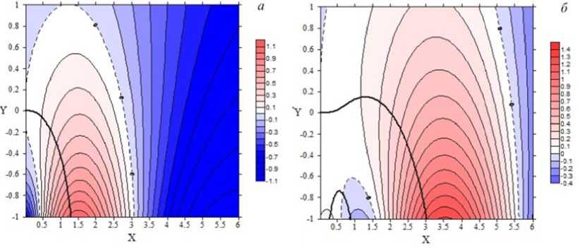
Figure 1. Solutions of dispersion relation (28) for various plasma parameters (in the parabolic approximation for the magnetic field): s’ / s0 = 0, n' / n = 0, s’ / s„ = 0, n‘ I n = 0, S=0 (а); s’ / s„ = 0, n' / n = 0, s’ / s„ = 0, 0p    0p          p p 0e0e          ee                      0p0p          pp          0e0e n‘ I ne = 0, S=1 (b). Here, X=Re (w/Hd ), Y=Im (w/Hd ), the isolines in the region of positive values correspond to Lb ЛN/ep ; the points of their intersection with the bold line, the solutions toN /Hd . The step of the change in Lb ЛN / Pp is represented to the right of each plot

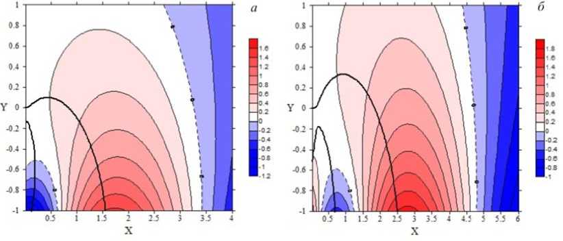
Figure 2. Same as in Figure 1 for the following plasma parameters: s’ /s„ = 0.3L \ n' /n = 0.3L-1, s’ /s = 1.5L1, pp           ee n' / n = -1.5L1, S=0 (а); s’ / s„  = 0.3L , n' / n  = 0.3L1, s’ / s„  = 1.5L ,  n' / n = -1.5L1, S =1 (b)

ee                   0_p0_p           pp           0_e0_e           ee

Neglecting the gradients, we get that the instability arises when S > to0 / Qd . For the chosen plasma e parameters it is easy to show that to0 / Qd > 1; e therefore, we determine the frequency ω0 and the instability increment γ, using Expressions (22) and (23) respectively. For small gradients, we obtain

f Lb„    )to0 =Qdp      ЛN l/( S + -),

\ ep      ) V 4 /

П

Y ^Q d .

^to 0

Q,

V d e

S + 5/ 2

_ ^to0 <  e ^de ,

V

S -^0- ^Q de

Г (S + 3/2)

The instabilit y occurs if i n model inver t ed electron dist r ibution (2) S > 59. For the c alculations, w e put S =60 (Figure 3). In t h is case, f ₀= 1 .6 mHz, th e increment Y = 4 .8 - 10 ^{- 5} s ^{- 1}, and Y/ f ₀=3^ 1 0^-2. Note th a t across the give n L-shell wit h the Alfvén velocity V A = 1000 km/s, the f undamental f requency of A lfvén reson a nce is ~7.7 mHz. Thus, the frequency o f the drift-co m pressional wave turns out t o be lower t h an the Alfvé n resonance frequency. At s m aller values of the azi m uthal wave nu m ber k ₂ , the d rift-compres s ional wave frequency is eve n less as be i ng directly p roportional to k 2 . The resulting ratio of t he incremen t to the eigen f requency is close to the values obtained in [Hughes et a l ., 1978] for Alfvén waves, ge n erated by th e bounce dri ft instability, and to the damping decrement o n the ionosp h ere.

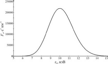
Figure 3. Model distribution functio n of hot electr o ns (2) with £ = 10 keV, в е =0.05, 5 =60 ^e max

CONCLUSION

The results allow us to co n clude that drift-compressional waves can propagat e not only i n the proton drif t direction (to the west) [C r abtree et al., 2 003, Klimushkin, Mager, 2011, Mager et a l., 2013], bu t also in the elec t ron drift direction (to the e ast). These w aves can also e x ist in the absence of plas m a temperatu r e and density gr a dients. In this case, the wave phase ve l ocity should be less than the mean particle magnetic drift velocity in the bump. Propagating i n the electro n drift direction, these waves can be increased due to res o nant interaction with electrons, i.e due t o drift insta b ility. This instability may develop at ce r tain electro n and proton te m perature and density grad i ents or beca u se of the inverted electron energy distributi o n.

For the magnetic shell L = 6 .6 R E , we have demonstra t ed that frequencies of d rift-compres s ional waves can be lower than eigenfrequ e ncies of ma g netic tube oscil l ations: at V _A=1000 km/s, the funda m ental frequency of Alfvén resonance is 7 .7 mHz, an d the drift-compressional wave frequency w ith the azi m uthal wave num b er k 2 =70 is 1.6 mHz. Because of the res o nant interaction of the wave with hot electrons, its amp l itude increases with an increment of 0.03 t o the frequenc y .

Our results can be helpful in interp r eting observatio n s of wave phenomena w ith frequenc i es in the range o f Pc5 geomagnetic pulsati o ns and belo w . For example, i n [James et al., 2013], Sup e rDARN dat a have been used to statistically analyze ULF oscill a tions occurring during substorm activity; i t has been s h own that in addition to the waves propag a ting in the p roton drift direct i on (to the west), there ar e waves runn i ng in the electron drift direction (to the e ast). In this case, periods of some of these waves c o nsiderably e x ceed those of P c 5 pulsations. Most likely t h ese waves a r e not Alfvén – they are probably drift-com p ressional, ru n ning in the ele c tron drift direction, and increased d u e to resonant interaction with energetic electrons in j ected into the m a gnetosphere during substo r ms.

The w o rk was supported by RFB R grant No. 16-05-00254a.