Driver behaviour profiling using dynamic Bayesian network

Published Online July 2018 in MECS DOI: 10.5815/ijmecs.2018.07.05

Driver behaviour analysis is an emerging trend for recent research. Detecting driving styles is essential towards improving on road safety. A vehicle driver’s driving style depends on a number of factors that include the state and nature of the road, the state of the driver, vehicle conditions and actions of other road users among other factors. Such driving styles may be characterized based on different factors that include overtaking, speeding, acceleration and braking trends.

Considerable research has been conducted in an attempt to monitor driver behaviour. Some of these studies demonstrated the use of self-reported data, human psychology data, Global Positioning System (GPS) data and Controller Area Network (CAN)-Bus data among others [1]–[8]. A 50 itemed Driver Behaviour Questionnaire was among the first techniques introduced in 1990 as a seminal article by Reason, Manstead and Stradling [5]. A Principal Component Analysis (PCA) on 520 drivers showed that errors were statistically distinct from violations, supporting the hypothesis that errors and violations are governed by different psychological factors [5]. De Winter and Dodou [4] recommended the questionnaire as a prominent measurement scale for examining driver’s self-reported aberrant behaviours as a predictor factor. Other approaches used different driver monitoring tools that operate either as roadside or on-board sensors. In such cases, unaware drivers can be monitored using roadside sensors, where various sensors can be used with the most common ones being cameras that track vehicle trajectories via image processing [3]. It is worth mentioning the DriveSafe [9] model, which is a smartphone app that collects driving manoeuvers data to evaluate, and profile drivers based on their behaviour. At the end of each trip, the driving behaviour is scored with trip records kept for the driver to analyse their skills and how to improve on them [9]. The goal behind the development of DriveSafe was to alert and assess driving behaviours to encourage safe driving and not to replace any onboard vehicle control system or driver assistance system [10].

Recent development in Intelligent Transportation Systems (ITS) is experiencing usage of both on-board and mobile devices that allow observations under more flexible experimental conditions, with the possibility of observing manoeuvers of particular interest in a controlled manner [3]. However, accuracy in the determination of driving styles for behaviour profiling is dependent on data analysis methodologies and techniques used.

This paper presents a model aimed at facilitating monitoring of a vehicle driver’s driving styles and nature of operational environment with respect to acceleration, braking and cornering trends using only data collected by a GPS on-board unit (OBU). To determine probabilities of different driver behavioural attributes and operational environment, Bayesian Networks are considered. The proposed model incorporates a notification module for sending driver behaviour profile messages via email and SMS at the end of the journey or day. The study was founded on GPS, GPRS, GSM and SMTP technologies. The proposed concept could be compared to the DriveSafe [9] model though using an OBU. In addition, it focuses on acceleration, braking and cornering as opposed to detecting inattentive driver behaviour as for the case of DriveSafe. Moreover, the model also determines the probability for the nature of operational environment with respect to road terrain and pattern.

The motivation behind this study was founded on the hypothesis that probabilistic methodologies are suitable for determination of driving styles and operational environments aimed at vehicle driver profiling. Furthermore, it is assumed that providing feedback of recorded driving actions to drivers could encourage a change of driving behaviour hence reduce individual risky behaviour. Full implementation of the proposed model could offer an affordable, easy to implement and operate solution that could find many applications in vehicle driver recruiting firms, vehicle insurance companies, government agencies and transport and safety industries. The model supports elements of Intelligent Transportation Systems.

The rest of the paper is organized as follows: section II presents contemporary studies on driver behaviour and profiling, section III outlines proposed model specification, section IV illustrates the design and implementation for the model, section V brings out results and their discussions and finally section VI concludes with suggestions for further work.

• II.    Related Work

A driver profile is a key performance indicator in the present world. Hence, mechanisms for profiling drivers based on their driving style are becoming a necessity in fleet management, automotive insurance and eco-driving [10]. Vehicle drivers operate under diverse and dynamic environments characterized by a number of factors. These factors in the context of the operational environment for vehicle drivers affects their behaviour. Theses includes familiarity of the environment, type of road, road pattern, terrain of the road, time of day, presence or absence of obstacles. Other factors that could be considered in the driver’s environment include the mechanical condition of vehicles, vehicle model, weather condition, driving region, state of the driver, state of other road users among others.

Notable contemporary studies have been carried out in an effort to monitor and analyse driver behaviour. For instance, Arroyo, Bergasa, and Romera [10] presented an adaptive fuzzy classifier for identification of sudden driving events based on acceleration, steering and braking styles using inertial and GPS smartphone in-built sensors. Just like in the case of [9], [12], the model by [10] detects acceleration and braking events based on sudden longitudinal changes measured by the accelerometer. The model [10] is composed of a fuzzy classifier that classifies events as acceleration, braking, steering and bumps centered on fuzzy logic and fuzzy rules without basing on fixed thresholds. A comparative experimentation of the DriveSafe [9] and the adaptive fuzzy model [10] saw the fuzzy model significantly reduce the number of false detections with considerable increase in real detections. Castignani, Frank and Engel [11] had early carried out an evaluation study of driver profiling fuzzy algorithms using GPS, accelerometer, magnetometer and gravity smartphone sensor. Their [11] proposed model puts all event types at the same scoring priority level merged in a global event counter. Sensor data from the smartphone is first filtered with events detected for the different metrics, followed by input data fuzzification with fuzzy rules applied in a Fuzzy Inference Engine [11]. Finally, a score is produced through a defuzzification process ranging from 0 to 100 [11]. A survey involving 20 drivers in different trips showed that drivers mainly belong to moderate and aggressive categories [11].

In the same line of adaptive fuzzy logic for driver profiling, Castignani, Derrmann, and Frank [13] proposed SenseFleet, a platform for driving event detection and scoring. The event detection algorithm used in SenseFleet uses accelerometer, gravity, magnetic and GPS smartphone sensors [13]. The model uses fuzzy logic to detect acceleration, braking and steering events [13]. These events are then combined with weather information and time-of-day through a scoring function for better determination of a score based on risky behaviour [13]. Using SenseFleet’s mobile application or a web-based dashboard, the overall score for all the trips and the relative distribution of event types can be analysed [13]. Each time an event is detected, a sound and text notification is triggered by the application as an instantaneous alert to the driver [13].

A more recent study by Obuhuma, Okoyo and McOyowo [14] explored mechanisms for providing real-time advisory alerts to drivers approaching mapped points of interest and/or experiencing overspeeding behaviour. The study [14] was carried out as a technical test of configurable technology supporting elements of Intelligent Transportation Systems, whose implementation could influence on driving behaviour, hence improving on performance and road safety. A text-to-speech Android app was used to read text SMS alerts to avoid diversion of driver’s attention [14]. Model validation experiments were limited to five points of interest namely, speed-limited zones, intersections, speed bumps, black spots and specific gas stations [14]. Such a model [14] is best suited to low-end infrastructure, common in developing nations.

The use of smartphones as a cheaper option compared to black-box on-board units is highly advocated by the DriveSafe model [9]. This is due to the high market penetration [10] of smartphones coupled with numerous sensors [11] emerging as a cost-effective means for capturing and processing real world data. For instance, the DriveSafe model is centered on a smartphone app [9] that requires the driver’s iPhone to be placed on the windshield, just below the rearview mirror and aligned with the relevant axes of the vehicle as a calibration mechanism. The app relies on inbuilt iPhone sensors for computer vision and pattern recognition techniques to detect the most commonly occurring inattentive driving behaviours. It detects two main categories of behaviour i.e. drowsiness and distractions [9]. Drowsiness is inferred based on lane weaving and drifting behaviours using rear cameras, microphone and GPS sensors [9]. In this case, lane weaving is detected if a driver changes lanes without turning blinkers while lane drifting is detected if a driver fails to keep the vehicle within the center of the lane [9]. Distractions are evaluated based on sudden longitudinal shifts indicated through acceleration, braking and turning events [9]. These measurements are established by the use of GPS, accelerometer and gyroscope iPhone sensors. Under normal circumstances, the accelerometer provides data in the range of -1 to 1 while the gyroscope data ranges between -180° to 180° [12]. Actual event detection depends on pre-processing of detected parameter that involves different mathematical functions and algorithms. The app then scores the driving behaviour based on the frequency and intensity of event detections with alerts presented to the driver on a Graphical User Interface (GUI) and alarms triggered upon exceeding of set thresholds [9]. The major limitation is the fact that the app only detects events at velocities higher than 50 km/h [9], [10].

Furthermore, the app majorly focuses on detection of drowsiness and distractions as opposed to the nature of operational environment.

The use of smartphones’ inertial sensors to detect driver behavioural parameters faces a number of challenges, two of which could have a great impact on the accuracy of the measurements [10]. Firstly, the diversity of the inertial sensors where measurements and noise level can differ among different devices. Secondly, smartphones position with respect to the relevant axis of the vehicle matters as a form of calibration. Hence, most modern day experiments [9], [12] for detecting driving events using inertial sensors use fixed thresholds to determine whether to report the event or regard it as noise. Accurate calibration is therefore required to establish these thresholds. These and many more factors make researchers continue basing their experiments on the use of both on-board units and smartphones with no major bias on either of the two.

Considering reviewed related studies, it is evident that most of the contemporary methodologies for profiling vehicle drivers based on acceleration, braking or speeding trends lack the element of notification to drivers upon completion of journeys. In addition, some approaches require lots of calibration during installation, hence, complex to implement and use. Furthermore, the use of fuzzy logic and fuzzy rules in detection and classification of driving styles featured in a number of studies. It is hence worth to explore other methodologies for profiling drivers based on driving styles. For instance, the use of probabilistic methodologies like Bayesian Networks. These and many other factors formed the basis and motivation behind this study.

• III.    Proposed Model Specification

This study proposes a cost effective, easy to implement model for profiling vehicle drivers based on acceleration, braking and cornering behaviour with notifications to drivers. The model aims to meet the following system requirements:

• 1)    Collect GPS data for a vehicle in real-time.

• 2)    Determine driving behaviour and operational environment probabilities per time-slice using Bayesian Networks.

• 3)    Generate a driver behaviour profile as a summary of behavioural and environmental probabilities for all time-slices for the entire journey.

• 4)    Send notifications to drivers bearing a summary profile for the journey.

• IV.    Design And Implementation

The proposed model comprises of four main sections: a central server, an instrumented vehicle, a driver with cellphone and GSM and GPS network services as outlined in the block diagram in Fig. 1.

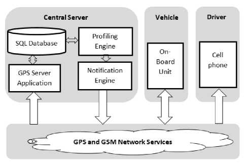
Fig.1. Proposed Block Diagram

• A.    Vehicle

Vehicle drivers operate under non-deterministic, unknown environments. A varied set of parameters is required to establish their behaviour. To affectively monitor the driver’s state of art with respect to the operational environment, an on-board unit is necessary. The study was established on an on-board unit that uses GPS technology to collect data from GPS satellites. GPS refers to a United States Government-operated network of earth-orbiting satellites that continuously provides time and position information to receiving stations and devices around the globe. There are approximately 24 active satellites participating in this network at any point in time. According to Yi, Li and Gu [15], GPS position is calculated using the concept of triangulation, using the known position of satellites overhead to determine the position of a GPS receiver pair on Earth. GPS receivers are positional speedometers that determine their speed using an algorithm that employs the doppler shift in the pseudo range signals from the satellites i.e. how far they moved since the last measurement [16]. The speed readings are updated at short intervals and normalized to maintain accuracy at all times, hence they are not instant speeds [16]. The Doppler shift is directly proportional to velocity of the receiver along the direction to the satellite, regardless of the distance to the satellite [16]. The receiver further transmits the data to the central server for processing using GPRS technology. The study proposes the use of GPS receivers that transmit data to the server in $GPRMC sentence format. The choice of the devices is informed by the required parameters that include vehicle speed, altitude, direction and a timestamp.

• B.    Central Server

The model has a central server consisting of four elements: a GPS server application, a profiling engine, a notification engine and an SQL-based database. The GPS server application receives GPS data from on-board GPS receivers fit in vehicles, processes the data then routes it to the database. The profiling engine generates drivers’ profiles by processing data stored in the database. A profile report is then routed to the notification engine for subsequent remission to the driver via either SMS or email. The study proposes an enhancement on the GPS server application developed by Obuhuma and Moturi [17] to incorporate the profiling and notification engines. The server [17] was developed based on socket programming technology using PHP with a MySQL database. Communication between the GPS receiver and the GPS server application is achieved through GPRS technology via a GSM network. The notification engine should use GSM, SMS technologies and the Simple Mail Transfer Protocol (SMTP) to facilitate sending of messages bearing driver profiles.

• C.    Driver

The model proposes that profile report notifications be send to drivers’ cell phones in form of SMS through GSM technology. This could be at any intervals, preferably at the end of a journey or day. To achieve better audit trails, a detailed copy of the SMS notifications to drivers could also be send to their personal email accounts at the end of the day with summaries, charts and links to map APIs for deep route analysis.

• D.    Profiling Metrics

The proposed model purely relies on only GPS data collected in realtime as drivers go along with their normal operations. The main parameters required for profiling drivers are speed, altitude, direction, timestamp and GPS signal strength data. A Driver’s position in form of coordinates is essential for the detailed report. The study proposes a driver’s profile for risk assessment founded on three main categories: acceleration, braking and cornering. The profiling engine determines a behavioural attribute to assign to the driver during each notification by establishing patterns for a given time period. Table 1 outlines possible behavioural attributes per category.

Table 1. Categories of Driver Behaviour Attributes

Profile Category	Behavioural Attribute
Acceleration	■    Normal Acceleration ■    Harsh Acceleration
Braking	■    Normal Braking ■    Harsh Braking
Cornering	■    Normal Cornering ■    Harsh Cornering

The study established no existence of world standard braking and acceleration metrics. However, some key metrics behind driver perception-reaction distance and braking distance that lead to a realisation of the stopping sight distance could be used in this case. Stopping sight distance is the distance covered during two phases of stopping a vehicle: perception-reaction time (PRT) and maneuver time (MT) [18]. Perception-reaction time is the time taken for a driver to realize that a reaction is needed due to a given condition, decides what maneuver is appropriate (in this case, stopping the vehicle), and starts the maneuver (taking the foot off the accelerator and depressing the brake pedal) [18]. On the other hand, maneuver time is the time taken to complete the maneuver (decelerating and coming to a stop) [18]. The distance driven during perception-reaction time and maneuver time is the Stopping Sight Distance (SSD) [18], expressed as:

SSD = (Perception-reaction Distance) + (Braking Distance) SSD = 0.278 Vt + (0.039 V2)/a (Metric)

SSD = 1.47 Vt + (1.075 V2)/a (US Customary)

Where:

• V – design speed in meter per second (m/s)

a – deceleration rate in meter per square seconds (m/s2)

t – brake reaction time, in seconds (s)

This may however vary because different vehicle models from different manufacturers have varied strengths and capabilities. For instance, some vehicles have powerful braking systems compared to others. Furthermore, other vehicles have greater power picking levels allowing instant speed shifts. The study hence proposes a braking and acceleration distance of less than 5 meters per square seconds to be normal. Any instances greater than this limit should hence be treated to be harsh acceleration or braking behaviour.

The model may be extended further to accommodate profiling for speeding as a category. In such cases, speeding profiling metric could be set to international or national standards. For instance, according to the Kenyan Traffic Act on speed limits, private motor vehicles are limited to 110km/h and 100km/h on dual carriageways and on single carriageways respectively. On the other hand, commercial vehicles, passenger vehicles, omnibuses and other public service vehicles are limited to 80km/h on all types of roads. Furthermore, speed limited zones require slightly low speeds. For instance, built up areas are always limited to maximum speeds of 50km/h or less regardless of type of road or vehicle.

• E.    Determination of Driver Profiles

The profiling engine utilizes graphical probabilistic models to establish the behaviour and nature of operational environment based on possible probabilities given a set of variables. The study was limited to four GPS data variables: speed, direction, altitude and signal strength against time. Two graphical models were considered: the Bayesian Network (BN) and the Dynamic Bayesian Network (DBN). The Bayesian Network is a probabilistic graphical model, a type of statistical model that maps a set of variables and their conditional dependencies. Bayesian classification theories are useful analyses forms for prediction of future data trends and intelligent decision-making [19]. Bayesian Networks are represented by a graph accompanied by a probabilities table. The graphical part of the Bayesian Network indicates the dependence or independence between variables hence providing an easy to comprehend visual knowledge representation tool [20]. On the other hand, the use of probabilities accommodates uncertainty in quantifying the dependencies between variables [20]. Fig. 2 outlines a Bayesian Network composed of four variables namely: speed, altitude, direction and GPS signal strength.

According to the graphical Bayesian Network, the driver profile depends on change in speed, altitude and direction. It is further evident that a change in speed is affected by changes in altitude and direction. Furthermore, the GPS signal strength affects changes in altitude, speed and direction. The probabilities in the network can therefore be summarized as:

P(Profile)  = P(∆Altitude | GPSSignal) . P(∆Direction |

GPSSignal) . P(∆Speed | ∆Altitude, ∆Direction, GPSSignal)

The possible driver profile observation can hence be represented in two sets: Behaviour and Environment sets as follows:

Profile={(‘normal_braking’, ‘harsh_braking’, ‘normal_acceleration’, ‘harsh_acceleration’, ‘normal_cornering’, ‘harsh_cornering’),

(‘meander’, ‘straight’, ‘up-hill’, ‘down-hill’)}

Based on the dynamic nature of GPS data against time, it is necessary to consider the Dynamic Bayesian Network representation. A DBN is a Bayesian Network that relates variables over adjacent time steps. It is hence often referred to as a 2-Time-slice Bayesian Network (2TBN). According to the 2TBN, at any given time t, the value of a variable can be calculated from the internal regressors and immediate prior value at time t-1. Fig. 3 illustrates the 2TBN for this case.

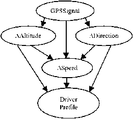
Fig.2. Bayesian Network for Driver Profiling

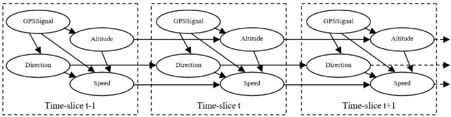
Fig.3. 2TBN for Driver Profiling

The model in Fig. 3 represents three copies of time-slices where each time-slice is a Bayesian Network. According to the network, the probabilities for the three time-slices can be summarized as:

P(Profile t-1 ) = P(Altitude t-1 | GPSSignal t-1 ) . P(Direction t-1 |

GPSSignal t-1 )   . P(Speed t-1    | Altitude t-1 ,

Directiont-1, GPSSignalt-1)

P(Profilet) = P(Altitudet | Altitudet-1, GPSSignalt) . P(Directiont | Directiont-1, GPSSignalt)  . P(Speedt | Speedt-1,

Altitudet,   Altitudet-1,   Directiont,   Directiont-1,

GPSSignal t )

P(Profilet+1)  = P(Altitudet+1  | Altitudet, GPSSignalt+1)  .

P(Directiont+1  | Directiont, GPSSignalt+1)  .

P(Speedt+1  | Speedt, Altitudet+1, Altitudet,

Directiont+1, Directiont, GPSSignalt+1)

This means that as time progresses, a new time-slice is generated. In which case, assuming good GPS signal strength, the value of each of the three GPS data variables is affected by the immediate previous value in the prior time-slice. There can be as many time-slices as the number of times the change in time is recorded. This model is hence vital for mapping of GPS data since such an analysis is a time series kind of analysis. It should hence be noted that a different profile for behaviour and environment is generated per time-slice. For effective driver profiling, an average of time-slice observations probabilities for a journey has to be determined by the profiling engine.

Such a DBN is defined as a pair, (BN, BN’), where BN is a Bayesian Network which defines the prior P(λ₁), and BN’ is a 2TBN that defines P(λ t | λ t-1 ) by means of a directed acyclic graph. This is as summarised in (1). Da et al. [19] present a deeper elaboration of the Bayesian Network model’s equation in a different way.

р(Л_£|Л_£ -1 ) = П^ 1 р(л ? |рг(Л ? ))         (1)

Equation (1) is referred to as a chain rule, where at any given time t, λ^k_t is the k’th node while Pr(λ^k_t) are its parents in the graph. The nodes in the first slice of a 2TBN are not associated with any parameters while each node in the second slice onwards has an associated conditional probability distribution, hence for all times t greater than 1, we define P(λ^k t | Pr(λ^k t )). It is worth noting that the parent of a node can either be in the same or previous time-slice. The complete joint distribution for j time-slices could hence be as defined in (2).

pUk’J) = П { ₌ 1 П^ 1 Р(я ? |рг(Л ? ))      (2)

• F.    Possible States with Profiling Probabilities

Table 2 outlines 64 possible states that each time-slice could fall under. The states have possible probabilities that the 2TBN could use to determine the behaviour and nature of the driver’s environment. A 2TBN is a generalization of the Hidden Markov Model (HMM). Hence, HMM could be applied to the states outlined in Table 2 to determine possible transitions and observation probabilities. However, this will result to a complex state diagram due to the high number of states and expected transition probabilities. Any additions of variables to the states, doubles or even triples the total number of probable states hence contributing to the complexity of the entire network. For instance, if we factor obstacles in the operational environment of the driver, then each of the current states will be duplicated to take care of presence or absence of obstacles. The set of states will hence shift from 64 to 128 states, complicating the network further.

• G.    Validation of Data Collection Tools and Method

To ensure consistency, accuracy and validity of data to be collected, data collection tools and methods should be validated. The study used the following validation process:

• 1)    The first step involved face validity through dialog and brain storming with experts in the transport and road safety industry and through research seminars. This led to the formulation of the driver behaviour and environment probabilities chart as outlined in Table 2.

• 2)    Based on validation test results outlined in [14] and the fact that the same tools and methods for data collection will be used in this study, the tests in [14] hence serve as a pilot study for the model proposed in this study. This serves as a test of validity for the data collection tools and consistency of data to be collected.

• 3)    Some revisions could be made to the data collection tools before full implementation of the proposed model. For instance, some thresholds may be adjusted in the driver behaviour and environment probabilities table if necessary.

The study was based on the assumption that, a horizontal GPS position accuracy of 5 meters is good enough to monitor and model driver behaviour with realtime tracking being some few seconds (approximately 3 seconds) behind the normal global time.

Table 2. Behaviour and Environment Probabilities per Driving State

	State				Behaviour						Environment
	∆Accl (m/s2)	∆Time (s)	∆Alt (m)	∆Dir (0)	Normal Accel	Harsh Accel	Normal Braking	Harsh Braking	Normal Cornering	Harsh Cornering	Meander	Straight	Up-Hi ll	DownHill
1	0 - 5	<=5	0 - 5	<+/-45	0.20	0.15	0.20	0.15	0.15	0.15	0.10	0.40	0.40	0.10
2	0 - 5	<=5	0 - 5	>=+/-45	0.20	0.15	0.20	0.15	0.10	0.20	0.40	0.10	0.40	0.10
3	0 - 5	<=5	> 5	<+/-45	0.25	0.10	0.25	0.10	0.15	0.15	0.10	0.40	0.50	0.00
4	0 - 5	<=5	> 5	>=+/-45	0.25	0.10	0.25	0.10	0.20	0.10	0.40	0.10	0.50	0.00
5	0 - 5	<=5	-0 - -5	<+/-45	0.25	0.10	0.25	0.10	0.15	0.15	0.10	0.40	0.10	0.40
6	0 - 5	<=5	-0 - -5	>=+/-45	0.25	0.10	0.25	0.10	0.10	0.20	0.40	0.10	0.10	0.40
7	0 - 5	<=5	< -5	<+/-45	0.20	0.15	0.20	0.15	0.15	0.15	0.10	0.40	0.00	0.50
8	0 - 5	<=5	< -5	>=+/-45	0.20	0.15	0.20	0.15	0.10	0.20	0.40	0.10	0.00	0.50
9	0 - 5	>5	0 - 5	<+/-45	0.25	0.10	0.25	0.10	0.15	0.15	0.10	0.40	0.40	0.10
10	0 - 5	>5	0 - 5	>=+/-45	0.25	0.10	0.25	0.10	0.12	0.18	0.40	0.10	0.40	0.10
11	0 - 5	>5	> 5	<+/-45	0.30	0.05	0.30	0.05	0.15	0.15	0.10	0.40	0.50	0.00
12	0 - 5	>5	> 5	>=+/-45	0.30	0.05	0.30	0.05	0.12	0.18	0.40	0.10	0.50	0.00
13	0 - 5	>5	-0 - -5	<+/-45	0.30	0.05	0.30	0.05	0.15	0.15	0.10	0.40	0.10	0.40
14	0 - 5	>5	-0 - -5	>=+/-45	0.30	0.05	0.30	0.05	0.12	0.18	0.40	0.10	0.10	0.40
15	0 - 5	>5	< -5	<+/-45	0.25	0.10	0.25	0.10	0.15	0.15	0.10	0.40	0.00	0.50
16	0 - 5	>5	< -5	>=+/-45	0.25	0.10	0.25	0.10	0.12	0.18	0.40	0.10	0.00	0.50
17	>5	<=5	0 - 5	<+/-45	0.05	0.30	0.05	0.30	0.15	0.15	0.10	0.40	0.40	0.10
18	>5	<=5	0 - 5	>=+/-45	0.05	0.30	0.05	0.30	0.10	0.20	0.40	0.10	0.40	0.10
19	>5	<=5	> 5	<+/-45	0.10	0.25	0.10	0.25	0.15	0.15	0.10	0.40	0.50	0.00
20	>5	<=5	> 5	>=+/-45	0.10	0.25	0.10	0.25	0.10	0.20	0.40	0.10	0.50	0.00
21	>5	<=5	-0 - -5	<+/-45	0.10	0.25	0.10	0.25	0.15	0.15	0.10	0.40	0.10	0.40
22	>5	<=5	-0 - -5	>=+/-45	0.10	0.25	0.10	0.25	0.07	0.23	0.40	0.10	0.10	0.40

23	>5	<=5	< -5	<+/-45	0.05	0.30	0.05	0.30	0.15	0.15	0.10	0.40	0.00	0.50
24	>5	<=5	< -5	>=+/-45	0.05	0.30	0.05	0.30	0.05	0.25	0.40	0.10	0.00	0.50
25	>5	>5	0 - 5	<+/-45	0.10	0.25	0.10	0.25	0.15	0.15	0.10	0.40	0.40	0.10
26	>5	>5	0 - 5	>=+/-45	0.10	0.25	0.10	0.25	0.18	0.22	0.40	0.10	0.40	0.10
27	>5	>5	> 5	<+/-45	0.15	0.20	0.15	0.20	0.15	0.15	0.10	0.40	0.50	0.00
28	>5	>5	> 5	>=+/-45	0.15	0.20	0.15	0.20	0.17	0.23	0.40	0.10	0.50	0.00
29	>5	>5	-0 - -5	<+/-45	0.15	0.20	0.15	0.20	0.15	0.15	0.10	0.40	0.10	0.40
30	>5	>5	-0 - -5	>=+/-45	0.15	0.20	0.15	0.20	0.10	0.20	0.40	0.10	0.10	0.40
31	>5	>5	< -5	<+/-45	0.10	0.25	0.10	0.25	0.15	0.15	0.10	0.40	0.00	0.50
32	>5	>5	< -5	>=+/-45	0.10	0.25	0.10	0.25	0.05	0.25	0.40	0.10	0.00	0.50
33	-0 - -5	<=5	0 - 5	<+/-45	0.20	0.15	0.20	0.15	0.15	0.15	0.10	0.40	0.40	0.10
34	-0 - -5	<=5	0 - 5	>=+/-45	0.20	0.15	0.20	0.15	0.20	0.10	0.40	0.10	0.40	0.10
35	-0 - -5	<=5	> 5	<+/-45	0.25	0.10	0.25	0.10	0.15	0.15	0.10	0.40	0.50	0.00
36	-0 - -5	<=5	> 5	>=+/-45	0.25	0.10	0.25	0.10	0.27	0.03	0.40	0.10	0.50	0.00
37	-0 - -5	<=5	-0 - -5	<+/-45	0.25	0.10	0.25	0.10	0.15	0.15	0.10	0.40	0.10	0.40
38	-0 - -5	<=5	-0 - -5	>=+/-45	0.25	0.10	0.25	0.10	0.25	0.05	0.40	0.10	0.10	0.40
39	-0 - -5	<=5	< -5	<+/-45	0.20	0.15	0.20	0.15	0.15	0.15	0.10	0.40	0.00	0.50
40	-0 - -5	<=5	< -5	>=+/-45	0.20	0.15	0.20	0.15	0.20	0.10	0.40	0.10	0.00	0.50
41	-0 - -5	>5	0 - 5	<+/-45	0.25	0.10	0.25	0.10	0.15	0.15	0.10	0.40	0.40	0.10
42	-0 - -5	>5	0 - 5	>=+/-45	0.25	0.10	0.25	0.10	0.20	0.10	0.40	0.10	0.40	0.10
43	-0 - -5	>5	> 5	<+/-45	0.30	0.05	0.30	0.05	0.15	0.15	0.10	0.40	0.50	0.00
44	-0 - -5	>5	> 5	>=+/-45	0.30	0.05	0.30	0.05	0.27	0.03	0.40	0.10	0.50	0.00
45	-0 - -5	>5	-0 - -5	<+/-45	0.30	0.05	0.30	0.05	0.15	0.15	0.10	0.40	0.10	0.40
46	-0 - -5	>5	-0 - -5	>=+/-45	0.30	0.05	0.30	0.05	0.25	0.05	0.40	0.10	0.10	0.40
47	-0 - -5	>5	< -5	<+/-45	0.25	0.10	0.25	0.10	0.15	0.15	0.10	0.40	0.00	0.50
48	-0 - -5	>5	< -5	>=+/-45	0.25	0.10	0.25	0.10	0.20	0.10	0.40	0.10	0.00	0.50
49	< -5	<=5	0 - 5	<+/-45	0.05	0.30	0.05	0.30	0.15	0.15	0.10	0.40	0.40	0.10
50	< -5	<=5	0 - 5	>=+/-45	0.05	0.30	0.05	0.30	0.20	0.10	0.40	0.10	0.40	0.10
51	< -5	<=5	> 5	<+/-45	0.10	0.25	0.10	0.25	0.15	0.15	0.10	0.40	0.50	0.00
52	< -5	<=5	> 5	>=+/-45	0.10	0.25	0.10	0.25	0.27	0.03	0.40	0.10	0.50	0.00
53	< -5	<=5	-0 - -5	<+/-45	0.10	0.25	0.10	0.25	0.15	0.15	0.10	0.40	0.10	0.40
54	< -5	<=5	-0 - -5	>=+/-45	0.10	0.25	0.10	0.25	0.25	0.05	0.40	0.10	0.10	0.40
55	< -5	<=5	< -5	<+/-45	0.05	0.30	0.05	0.30	0.15	0.15	0.10	0.40	0.00	0.50
56	< -5	<=5	< -5	>=+/-45	0.05	0.30	0.05	0.30	0.20	0.10	0.40	0.10	0.00	0.50
57	< -5	>5	0 - 5	<+/-45	0.10	0.25	0.10	0.25	0.15	0.15	0.10	0.40	0.40	0.10
58	< -5	>5	0 - 5	>=+/-45	0.10	0.25	0.10	0.25	0.20	0.10	0.40	0.10	0.40	0.10
59	< -5	>5	> 5	<+/-45	0.15	0.20	0.15	0.20	0.15	0.15	0.10	0.40	0.50	0.00
60	< -5	>5	> 5	>=+/-45	0.15	0.20	0.15	0.20	0.27	0.03	0.40	0.10	0.50	0.00
61	< -5	>5	-0 - -5	<+/-45	0.15	0.20	0.15	0.20	0.15	0.15	0.10	0.40	0.10	0.40
62	< -5	>5	-0 - -5	>=+/-45	0.15	0.20	0.15	0.20	0.25	0.05	0.40	0.10	0.10	0.40
63	< -5	>5	< -5	<+/-45	0.10	0.25	0.10	0.25	0.15	0.15	0.10	0.40	0.00	0.50
64	< -5	>5	< -5	>=+/-45	0.10	0.25	0.10	0.25	0.20	0.10	0.40	0.10	0.00	0.50

• V. Results and Discussion

An on-board GPS receiver was used to collect and log 230 data points at the GPS server for a sample experiment whose route map is as outlined in Fig. 4. The experiment was carried out on a dual carriageway road segment. The road segment was familiar to the driver. It was composed of relatively straight stretches with few clear corners controlled by roundabouts. The road terrain was relatively flat with a gentle slop at some point. Other factors included daytime, dry weather, a mixture of both built-up and nonbuilt-up sections. Fig. 5 – 9 outlines summaries of experiment results.

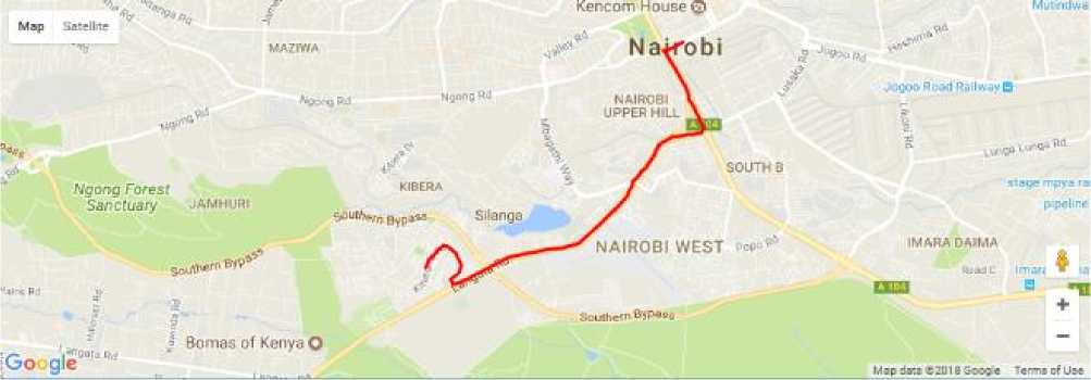
Fig.4. Route Map for a Sample Experiment

Acceleration/Deceleration (m/s2)

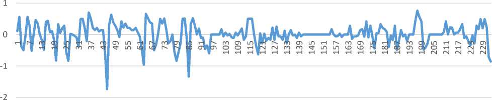
Fig. 5. Patterns for Acceleration and Deceleration

Speed (km/h)