Dynamic Passenger OD Distribution and System Performance of Taxi Operation System

Published Online March 2011 in MECS

In most urban areas, taxis are an important means of public transportation for that they provide a speedy, comfortable, door-to-door and 24-hour available transportation service. However, as a taxi can serve only single or a small number of passengers, this inefficient transportation facility greatly adds to road traffic congestion. Therefore, taxi services are subject to various types of regulation. Regulators hope to give attention to both system efficiency and service level, so that taxis may share a rational part of urban travel demand and benefit both operators and customers. Effective intervention depends on suitable regulatory information, involving an evaluation of the impacts of such intervention on the demand and supply and the level of taxi services [1]. It is thus of strong interest to model the dynamic process of taxi services from both a theoretical and a practical point of view.

The economics of taxi services have been emphasized by a number of authors using descriptive conclusions.

Supported by “Research Fund for the Doctoral Program of Higher Education of China” (20100205110004), “the Fundamental Research Funds for the Central Universities” (CHD2009JC059)

They found that: (a) the demand for and supply of taxi service are interrelated through the role of intervening variables of passenger waiting time and taxi occupancy; (b) in equilibrium, the quantity of service supplied (vacant and occupied taxi hours) will always be greater than quantity demanded (occupied taxi hour); (c)this amount of slack (vacant taxi hours) produces an upward pressure on service price that drives the system to a condition with high fares, low cab occupancy, low passenger waiting times and price competition none existent;(d) regulations have been recommended and adopted almost everywhere, while fare and entry regulations have been emphasized as the most commonly considered interventions by different authors. These conclusions are mainly derived from simplified, abstract and aggregate models, and stem from assumptions that taxis are operating under homogeneous conditions such that all taxis have the same number of passengers, passenger trips have the same lengths, taxi speed is uniform, and the passenger locations in the city are homogeneous etc. [2-6]

However, the uncertainty and dynamic features of taxi operation system are not concerned and the impact of vacant taxi behavior still cannot be obtained precisely from these models. As a result, it is difficult to determine average passenger waiting time, the most important measurement for service level. Most previous studies simply use or develop the idea of Douglas[7], who made reference to Mohring[8] in which an analogous result was obtained for bus travel. Douglas’ model of vacant taxi search can be summarized by:

V = N - Qt (1)

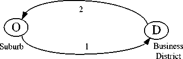
Figure 1. A specific structure w = w (V) =

A

Vs

A

5 ( N - Qt )

where N is the number of taxis, Q is the demand for taxis and t is average passenger trip time. Thus Qt denotes the occupied taxi hours and V denotes the number of vacant taxis. A is the number of street kilometers and s is the average taxi speed, w is the average passenger waiting time. As is mentioned above, the operating conditions are supposed to be homogeneous. However, (2) is more likely to illustrate average vacant taxi headway than average passenger waiting time. We doubt whether it is suitable to measure average passenger waiting time in a real urban environment where the operating conditions are usually not that homogeneous.

Fig.1 presents a specific city structure of taxi operation system. We use such a specific structure simply because this system can be explained not only by classic taxi theory, but also another classic method: queuing theory. With the latter, it is possible to verify the result of (2). It is supposed that N = 5 taxis are operating in the system. During the morning rush hour, Q = 12 passengers would start from suburb O to business district D in 1h. After picking up a passenger from node O , the taxi will move to D by link 1. And once a customer ride is completed at D , the taxi will go back to O by link 2 to search for new passengers. Each link has the same length of 3 km, which is A = 6 km. The average taxi speed is supposed to be 5 = 60 km/h. Then, according to (2), the average passenger waiting time is:

w =--------= 0.0227h = 1.36 min     (3)

5 ( N - Qt )

However, if we suppose that the passenger arrivals occur according to a Poisson process, with passenger arrivals X = Q = 12 , and link travel time is exponentially distributed, this system turn out to be an M/M/5 queuing system. As a taxi will return to O for new passengers after sending a passenger to D , the maximum service capacity of a taxi is ц = 60/(3 x 2) = 10 . Then from Little’s result[9], we have:

P 0 =

N - ( N p ) k + ( N p ) ^N ' Ь k ! N !(1 - P ).

- 1

= 0.3011

L   ( ^N P ) NP ₀

w = — =---------—

^X   ^ n n N !(1 - p )²

= 0.216 x 10 ³h=0.013min (5)

where p ₀ is the probability of finding no passengers in the system , p = X /( N ^ ) = 0.24 , L is the average number of passengers in the queue. It is shown that average passenger waiting time obtained by queuing theory is only about 0.013min. The error between 1.36min and

0.013min is big enough to bring about improper interventions. Therefore, more accurate methods should be developed to determine average passenger waiting time of urban taxi operation system.

In view of the fact that demand for and supply of taxi services take place over space, Yang, Wong and their colleagues developed a series of network models to analyze the supply-demand equilibrium characteristics of cruising taxi services for the case of Hong-Kong[10-13]. They supposed that once a passenger ride is completed, the driver would decide whether to stay in the present zone or go to another zone to search for passengers. The probability that a taxi go to each zone is specified by a logit model. They contribute greatly to the study of vacant taxi behavior in detail. However, as is still a stationary study, their vacant taxi model has some limitations. First, the decision-after-passenger-arrival assumption makes a direct connection between the number of passengers and the number of vacant taxis in the streets, which lead to a confusing result that average vacant taxi headway is irrespective of taxi fleet size[10]. As is common sense, if there are more taxis operating in a city, more vacant taxis will appear and the average vacant taxi headway should be smaller. Second, once a taxi at zone i decided to go to another zone j , this decision will never change until the taxi finds a new passenger in zone j . That is, the taxi will pay no mind to passengers in a midst zone between i and j as it passes by. And if there are no passengers in zone j , the taxi will stay there in vain. In reality, taxi drivers may change their decision with respect to driving experience and available information. They will pick up passengers they meet no matter in zone j or anywhere else. And if they expect long search time at one place, they will drive to other places. This dynamic vacant taxi behavior is an important feature of taxi operation system and exerts great influence to system performance. And the third, as average passenger waiting time cannot be determined directly from their model[10], they go back to Douglas when determining the average passenger waiting time [11, 12].

In China, cruising taxi service is the predominant mode of taxi operation system. Vacant taxis cruise in the city to search for passengers and accept street hails. Passengers may start at any place of a street, and taxis may stop and pick up passengers anywhere along roadside. Therefore, it is necessary to pay more attention to the randomness of the appearances of passengers. This paper considers urban taxi operation system as a special structure queuing system, and proposes a discrete event simulation model. It is supposed that a passenger trip may start from or end at both the nodes and links in the city, and taxis decide where to find new passengers mainly based on driving experience and available information. The model attempts to deal with the dynamic performance of taxi services. Through a simulation experiment, the 24-hour time-variant features of taxi services can be obtained and a new method of determining optimal taxi fleet size is proposed. These are helpful to taxi operators for raising their efficiency and supervisors for providing better services.

• II.    The modeL

A.    Basic Assumptions and Logical Structure

• 1)    Nodes, links and segments

Consider that there are N taxis operating in an urban network G ( V , A ), where V is the set of nodes and A is the set of links. Passengers may start from and end at any places in the city, both nodes and links. Nodes denote taxi stands where there are some parking spaces that taxis can wait for passengers there. In a city, such places may be airport, train station and etc. Long taxi queues and mass of passengers are often observed at these places. Taxis take turns to pick up passengers and only when there are no taxis waiting, do passengers need to stand in a line to wait for service.

Links denote streets connecting those nodes. When a passenger arrives at a street, he just hails a taxi as it goes by. Taxis are permitted to stop at streets to pick up or release passengers, but there is no space for taxis to wait and they must leave quickly. Each link is divided into a certain number of segments, and each segment is considered to be a taxi stand where taxis can not line up and wait for passengers.

• 2)    Queuing discipline and Fare structure

In real taxi operation system, it is often observed that when a passenger arrives at airport or train station, he usually takes the first taxi from the taxi queue, and if passengers need to wait for taxis, they also have to take turns. So the queuing discipline at these places is supposed to be first-come-first-serve (FCFS). While at streets, it is often observed that several passengers vie with each other for the same taxi. Thus the queuing discipline at these places is supposed to be random order of service (ROS).

Fare of taxi service often comprises a fixed initial hiring charge and a distance charge. For simplicity, a time charge is not considered here. Thus price passenger m is:

F_m for

f

F = <      0

m   1 f0 + f. ( s.

, s m <  s 0

s 0 )    , s m ^ s 0

where f ₀ is the initial charge for the first s ₀ kilometers, f ₁ is the distance charge, s_n is the passenger trip distance.

• 3)    Logical structure

In this paper, taxi operation system is considered to be a special structure queuing system. This system possesses features as follows. (i) the servers are moving in a road network to provide travel services, while in ordinary queuing systems, the servers are immobile; (ii) not only passengers are in queues waiting for services, but the taxis are often observed to be lining up to wait for passengers; (iii) the servers have the ability to search for customers, (iv) a passenger’s trip time is affected greatly by road traffic congestion.

г

Data Initialization

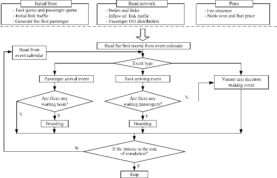
Figure 2. Logical structure of the model

In order to deal with these dynamic features of taxi services in an urban network and consider the uncertainty in both demand and supply, we develop a discrete event simulation model, in which taxi services are described with four kinds of event: passenger arrival event, taxi arriving event, boarding event and vacant taxi decision making event. The passenger arrival, taxi arriving and vacant taxi decision making events are scheduled in the event calendar, while the boarding event happens after passenger arrival or taxi arriving event. Fig.2 is the simulation framework of the model.

The simulation begins in an “empty-and-idle” state. That is, no customers are present, and taxis are vacant and waiting at those nodes. Then, at time 0, the first passenger is generated. Detailed process of those events will be introduced respectively in the following part of this section.

B.    Passenger Arrival Event

Passenger arrival event is mainly concerned with three problems. First, it is to be determined the passenger’s origin place and destination. Second, what will the passenger do after coming to the origin place? Third, the next passenger arrival event has to be scheduled in event calendar.

Suppose that o_ij , which is given, denotes the number of passengers starting from origin place i to destination j within a simulation minute. Thus O i = ^ j o i denotes the number of passengers starting from origin place i . Then, when a passenger arrivals, the probability of the origin place to be i is:

p    i °O                ⁽⁷⁾

k e S

After the origin place is determined, the probability of the destination to be j is:

o

P D, = O               <⁸

If the origin place is a node, the passenger will check whether there are any taxis waiting. If so, the passenger will select a taxi and boarding event will be invoked. If there are no taxis waiting, the passenger would be p into the passenger queue of the origin place. The flowchart of the passenger arrival event is depicted in Fig.3.

C.    Taxi Arriving Event

This event imitates the taxi arriving process with respect to the state of the taxi, that is, whether the taxi is occupied by a passenger. The arriving of an occupied taxi is, in other words, the departure of the passenger. After the passenger gets off, the taxi will become vacant. Then it turns out to be the same with the vacant taxi arriving event. A check is made to determine whether there are passengers waiting. If so, the vacant taxi will pick up a passenger from the passenger queue. Then boarding event is invoked.

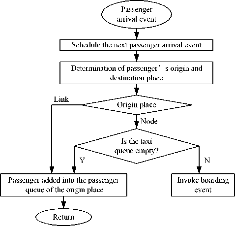
Figure 3. Passenger arrival event

If there are no passengers waiting, the taxi has to determine where to search for passengers and the vacant taxi decision making event is invoked. Detailed process of this event is depicted in Fig.4.

D.    Boarding Event

The primary mission of this event is to determine the service time of a passenger trip and schedule corresponding occupied taxi arriving event. As is mentioned above, the taxi is supposed to move to the passenger’s destination via the shortest path. The service time of a passenger trip depends on the customer’s trip distance, and is influenced by link traffic flow. Suppose that the taxi drives to the passengers destination via link l , then the travel time t_nl on link l can be determined by the following Greenshields equation[14].

Lnl tnl vl

v_l min

L_{nl |} max ^ min-

)[1 - (-f^)“ ]e d ljam

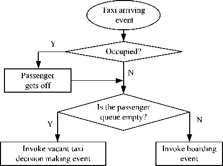
Figure 4. Taxi arriving event where Lnl is the passenger’s travel distance on link l , vl is taxi speed, vlmin is the minimal speed on link l ,while vlmax is the free speed. dl is the traffic flow at current time on link l , while dljam is the max traffic flow on link l .

E.    Vacant taxi decision making event

Taxi drivers can’t tell exactly where they can find new passengers, but an experienced driver does be able to perceive the passenger arrival rate of those nodes and segments. Therefore, he will do decision based on his driving experience. This event imitates drivers’ decision making process.

At a segment with no parking space to wait for passengers, the search behavior is quite simple: drivers just need to move on to the adjacent segment of the link. If the taxi is at a node, the driver’s decision making is illustrated through three steps.

First, he would estimate the expected waiting time at present node according to the quantity of vacant taxi and passenger arrival rate.

Suppose that there are x vacant taxis at present node i , and the passenger's arrival rate from the driver’s perspective is a . If the queuing discipline is FCFS, and there are x ₁ taxis ahead, then the expected search time would be x ₁ / c .

If the queuing discipline is ROS, suppose x ₂ denotes the vacant taxis at present node. Then the probability that the taxi will meet a passenger after waiting for t minutes would be:

P. = ^- (1 - ^- ) t ^{- 1}

x ₂ x ₂

Therefore, the expected search time would be determined by the following mathematical expectation:

”       ”

w. = L p = £ t - (1 - - )⁽ t ^{- 1)} = x 2

t = 0        t = 0   x 2       x 2           -

Second, he would estimate the expected search times if goes to the other nodes according to driving experience and the available supply-demand information along the road network. Suppose that l is a link that connects present node, and the driver assumes that it would take as long as the mean of the taxi’s previous search times that he meets a passenger on link l .

The third, the driver would select the target of the minimum expected search time.

• III.    Target of simulation

Regulations should be judged by the predicted effect of changing it. Therefore the target of this paper is: 1. to quantitatively determine system performance metrics, and 2. to develop a method for the solution of system optimal taxi fleet size.

A.    System performance metrics

In this paper, metrics examined to evaluate system performance of taxi services include average taxi occupancy, average vacant taxi travel rate, average taxi income, profit and fuel cost, average passenger waiting time and average vacant taxi headway.

Taxi occupancy and vacant taxi travel rate are important indices about service utilization. Taxi occupancy is the ratio of total occupied taxi-hours to total taxi-hours in services, while vacant taxi travel rate is the ratio of vacant travel taxi-hours to total taxi-hours. Total taxi-hours consist of the occupied taxi-hours, vacant travel taxi-hours and vacant waiting taxi-hours. We only examine the occupied and vacant travel taxi-hours here, and the ratio of vacant waiting taxi-hours can be determined by them. High taxi occupancy, low vacant taxi travel rate are wanted by taxis proprietors. Taxi income, profit and fuel cost are indices which directly describe the living conditions of taxi operators.

Average passenger waiting time and vacant taxi headway are important metrics of service level. Average passenger waiting time means how long a passenger would take to wait for a taxi. Vacant taxi headway is the time interval between two adjacent vacant taxis, which is a closely relevant measurement of taxi availability. It is obvious that low passenger waiting time and low vacant taxi headway are wanted by passengers.

B.    Determination the social optimal taxi fleet size

The first best optimum of taxi operation system is derived by minimize social cost[3,5,15], which is made up of total passenger cost and total taxi cost.

min J = £ C m .^: ⁽¹²⁾ mn

Where C m denotes cost of passenger m , and T n denotes cost of taxi n. C_m can be obtained by following equation.

C m = ^F m ⁺ a ⁽ h m ⁺ w m )

f f 0 + a ⁽ h m ⁺ w m ) s m <  s 0 ⁽¹³⁾ [ ^f 0 + / 1 ⁽ s m - s 0 ) ⁺ a ⁽ h m ⁺ w m ) s m ^ s 0

Where F_m is the payment of passenger m , which is defined in (6). h_m denotes the passenger trip time, while w_m denotes the passenger waiting time. a is the value of time from the passenger’s perspective.

T n can be obtained by following equation.

T n =-r_w = C n 1 + C n 2 - R n (14)

n _n is the profit of the taxi n. C n 1 and C n ₂ denote the fixed and variable cost of the taxi. R_n is the income of the taxi within study time period. C_{n 1} consists of license fee, depreciation, maintenance cost, drivers’ salary and etc, which can be obtained from statistic data. C_{n 2} consists most of the fuel cost, which can be obtained by fuel price multiplied by taxi kilometers within the studied period.

Since all passengers’ payments turn out to be the total income of all the taxis, we have optimal objective function as:

min J

= Z F m + Z a ( h m + W m ) + £ ( C n 1 + C n 2 ) - Z ^ n (15) mm     n     n

= Z a (h m + W m ) + Z ( C n 1 + C n 2 )

• IV.    Simulation example

This example studies the time variant features of taxi operation system. The city is depicted in Fig.5(a). Link data is presented in Table 1. Each link is divided into a number of segments with the length of each segment to be 0.25km and sum up to total 264 segments. Therefore, there are totally 268 taxi stands in the city as is depicted in Fig.5(b). Stands 1-4 denotes those nodes, and 5-268 are those segments. At stands 1 and 2, which may be airport and the train station, the queuing discipline is supposed to be FCFS, while at other stands, the queuing discipline is ROS. The 24-hour in a day is divided into 96 time periods with each period to be 15 minutes. It is supposed that passenger arrival rate within each time period is a constant, and the passenger distribution within 24-hours is depicted in Fig 6.

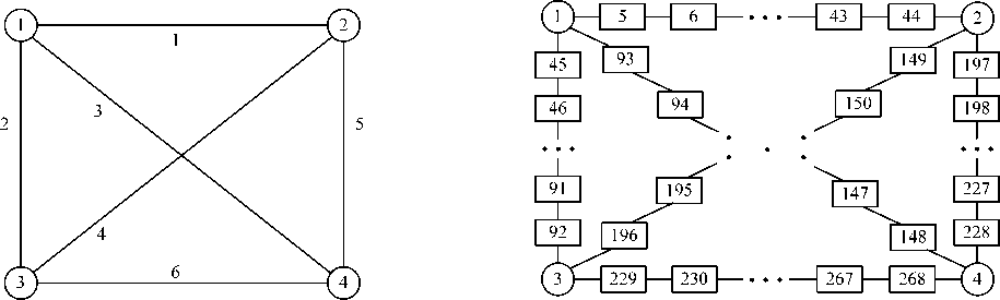
(a) Urban road network                                       (b) Nodes and segmengs of the links

Figure 5. Network used for numerical example

TABLE I.

L ink data

Link number	Nodes connected	Length (km)	Number of segments	direction
1	1-2	10	40	1→2 2→1
2	1-3	12	48	1→3 3→1
3	1-4	14	56	1→4 4→1
4	2-3	12	48	2→3 3→2
5	2-4	8	32	2→4 4→2
6	3-4	10	40	3→4 4→3

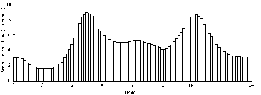
Figure 6. 24- hours passenger distribution

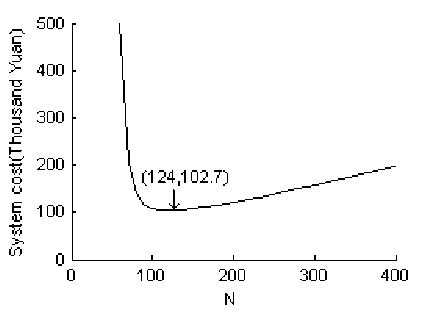
Figure 7. System cost and social optimal taxi fleet size

Determining the taxi fleet size of a city is one of the most important subjects of the regulators. According to (15), we propose a simulation method to determine social optimal taxi fleet size. Fig.7 is the simulation result of total system cost with varied taxi fleet size. It is shown that with the growth of the number of taxis operating in the system, system cost curve firstly decreased sharply, and then slowly increased. As is mentioned above, system cost is made up of passenger trip time cost and total taxi operation cost. With the growth of the number of taxis operating in the system, average passenger waiting time decreases sharply, and at the same time, taxi operation cost increases. The impacts of both result in the existence of the minimum system cost, and the taxi fleet size of the minimum system cost is the social optimal taxi

Hour

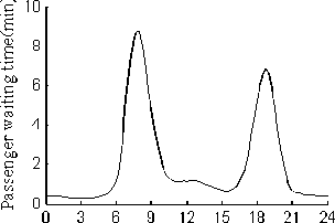
(a) Passenger waiting time

Figure 8. Taxi service utilization under homogeneous situation

fleet size. In this experiment, it is 124 taxis and the system cost is 102.7 thousand Yuan a day.

Under the social optimal taxi fleet size 124, simulation experiments are carried out to examine the time variant features of system performance measures. Fig8 is the simulation results of service level. Corresponding to dynamic taxi demand, these measures are time variant and differ greatly at different time period. It is shown that at peak hour, average vacant taxi headway is about 4-6min, and average passenger waiting time is even as higher than 8 minutes in the morning rush hour. It means that at peak hours, it is quite difficult for a passenger to find a vacant taxi.

Fig.9 is the time variant features of system operation efficiency with taxi fleet size to be 124. It is shown that at peak hours such as 7-8 in the morning and 18-19 in the evening, taxi occupancy rate is nearly 80%, while vacant taxi travel rate is no more than 10%. Average taxi income is much more than fuel cost, drivers have good profit. At midnight, only a small part of taxis are occupied. However, in this experiment, although profit is negative, taxi income is still higher than fuel cost and can cover a certain part of fixed cost. Therefore, drivers would still keep on working. If taxi income is lower than fuel cost, it means operating a taxi is completely running at a loss, and the driver would go back home and sleep at that time period.

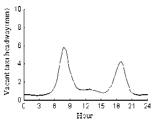
(b) Vacant taxi headway

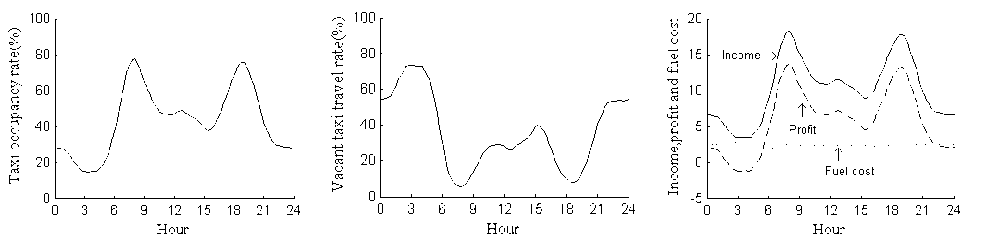
(a) Taxi occupancy rate                      (b) Vacant taxi travel rate                (c) Income, profit and fuel cost

Figure 9. Taxi service utilization under mixed situation

• V.    Conclusion

This paper put forward a discrete event system simulation model of the taxi service system in a dynamic road network. A new method of determining social optimal taxi fleet size is proposed, and the 24-hour time variant features of system performance can be recurred. It is shown that considering the time-variant effect can help to get more accurate information about the taxi services. Further study is being undertaken to consider more detailed factors, such as signals and drivers’ speed preference. The effect of price interventions and entry restriction are to be studied.