Economic and Statistical Modelling of Production Processes in the Regions of the Arctic Zone of the Russian Federation

DOI:

Economic and statistical modeling of phenomena and processes in regional systems is an important area of research within the framework of regional economics. Obviously, it is associated with the urgent need to study the quantitative side of regional phenomena and processes conditioned by their qualitative characteristics, to understand the patterns of social development, to quantitatively assess the interrelations of economic phenomena and processes, and to substantiate the forecast of the development of regional systems. The drawbacks and limitations of the application of modelling to real data, including at the regional level, are much less discussed. However, a number of researchers, including the authors of this article, have devoted a series of publications to discussion of this issue [1, pp. 9–14, 59–65; 2–7]. We believe that such publications were useful because, among other things, as V.N. Novoseltsev and Zh.A. Novoseltseva rightly point out, “besides errors of the modelling method itself, there are also errors related to the qualification of researchers. They are not inherent to models as such, but are, perhaps, a reflection of insufficient attention of researchers to the model being created” [8].

One of such shortcomings is underestimation of the specifics of real economic processes caused not so much by intraregional factors of the regional system functioning as by external control influences that distort the behavior of the system and its components so significantly that it complicates and/or makes impossible the application of typical economic and statistical models that work well in standard economic regional systems. For example, our previous studies have shown that the statistically confirmed specifics of the functioning of the economies of the Northern and Arctic regions [9; 10] can limit the possibilities of using production functions (PFs) due to the imbalance in the behavior of the main production factors [11; 12].

PFs, despite their known limitations, are traditionally widely used as a research tool not only in scientific studies, but also in domestic and foreign management practice, including in official forecasts of the development of countries and regions [13, pp. 119–134; 14]. This is due to the fact that they are a convenient tool for analysis and forecasting, displaying the relationship between the physical volume of production factors and the physical volume of output in the process of producing goods or services. It is also important that PFs, as a rule, “work” well on real data. In this regard, it is of interest to construct PFs for the regions of the Arctic Zone of the Russian Federation, taking into account possible limitations of their use in a number of regions of the Arctic Zone of the Russian Federation. Thus, the purpose of the study is economic and statistical modelling of production processes in the regions of the Arctic Zone of the Russian Federation using PF tools.

Initial data and assessment of the possibilities of constructing models of production functions for regions of the Arctic Zone of the Russian Federation

As noted, our previous studies have shown that the specifics of functioning of the economies of the North and Arctic regions can limit the possibilities of using PFs due to the unbalanced interaction of the main factors of production [11; 12]. Therefore, at the preliminary stage, a de-

SOCIAL AND ECONOMIC DEVELOPMENT

Sergey V. Baranov, Tatiana P. Skufina. Economic and Statistical Modelling … tailed correlation and regression analysis was carried out, establishing the interrelations in the behavior of production factors in the regions of the Arctic Zone of the Russian Federation. In order to present the all-Russian situation, the Russian Federation as a whole was also considered.

The following data for 2000–2021 were used in the work: the index of physical volume of the GRP of the Russian Federation in constant prices as a % of the previous year, adjusted to the values of 2000; the index of physical volume of investments in fixed capital (IFC) in comparable prices as a % of the previous year, adjusted to the values of 2000; the fixed assets value (FAV) at the end of the year at full accounting value taking into account the degree of depreciation, adjusted to the values of 2000 using the GDP deflator index; the degree of depreciation of fixed assets (at the end of the year; in percent); GDP deflator indices; the average annual number of people employed in the economy of the Russian Federation, adjusted to the index form relative to 2000 (number of employees, NE).

The analysis of the dynamics of GRP, investment in fixed capital, the value of fixed assets and the number of people employed for 2000–2021 (Fig. 1, 2) showed that there are significant differences in the behavior of these indicators. In particular, in a number of regions (the Republic of Karelia, the Komi Republic, the Murmansk Oblast, the Krasnoyarsk Krai and the Chukotka Autonomous Okrug), the changes in GRP and the number of employed demonstrate opposite dynamics. In order to quantitatively characterize this feature, the Pearson correlation coefficients between GRP and production factors were calculated: GRP and investment in fixed assets, GRP and the value of fixed assets, GRP and the number of employed (Table 1). Based on the analysis of correlations, the studied regions were divided into 3 groups.

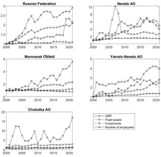
Fig. 1. Dynamics of GRP production factors for 2000–2021 for the entire Russian Federation and regions that are fully included in the Arctic Zone of the Russian Federation. The values of the indicators (GRP, value of fixed assets, investment in fixed capital, number of employees) were used in the indices of physical volume in comparable prices.

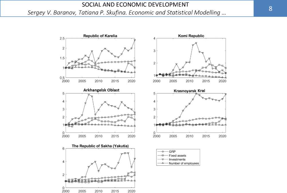
Fig. 2. Dynamics of GRP production factors for 2000–2021 for regions that are partially included in the Arctic Zone of the Russian Federation. The values of the indicators (GRP, value of fixed assets, investment in fixed capital, number of employees) were used in the indices of physical volume in comparable prices.

Table 1

Pearson correlation coefficients between GRP and production factors for 2000–2021. Between GRP and investment in fixed capital (IFC), GRP and fixed assets values (FAV) of economic sectors, GRP and number of people employed in the economy (NE) 1

Region	GRP-IFC	GRP-FAV	GRP-NE	GRP-NE	IFC-NE
Russian Federation	0.98	0.73	0.86	0.64	0.77
Fully in the AZRF
Murmansk Oblast	0.73	0.56	-0.59	-0.88	-0.90
Nenets AO	0.65	0.81	0.93	0.80	0.70
Chukotka AO	0.56	0.54	-0.08	-0.33	0.06
Yamalo-Nenets AO	0.88	0.94	0.95	0.92	0.89
Partly in the AZRF
Arkhangelsk Oblast	0.67	0.84	-0.69	-0.62	-0.08
Krasnoyarsk Krai	0.94	0.56	-0.42	-0.81	-0.32
Republic of Karelia	0.77	-0.11	-0.49	0.49	-0.69
Komi Republic	0.87	0.18	-0.23	-0.84	-0.13
Republic of Sakha (Yakutia)	0.89	0.75	0.89	0.72	0.91

Group 1 includes entities in which the mutual behavior of the main production factors (labor and capital) fits into generally accepted concepts: there is a significant positive relationship between GRP and production factors. Group 1 includes: the Russian Federation as a whole, the Nenets Autonomous Okrug, the Yamalo-Nenets Autonomous Okrug, and the Sakha Republic (Yakutia). For these regions, it is possible to construct classical models of GRP production in the form of production functions.

• ¹    Values of indicators were used in physical volume indices in comparable prices.

Group 2 — entities in which the mutual behavior of the main production factors does not fit into classical concepts: there is a sufficiently strong positive relationship (the square of the correlation coefficient is not less than 0.6) with only one of the production factors. For example, the GRP of the Arkhangelsk Oblast (Table 1) has a sufficiently significant positive relationship with the value of fixed assets (GRP-FAV = 0.84) and a negative relationship with the number of employees (GRP-NE = -0.69). Group 2 includes: the Arkhangelsk Oblast, the Krasnoyarsk Krai, and the Komi Republic. For each region of this group, a single-factor model was additionally constructed, which included a factor with a positive relationship with GRP.

Group 3 — entities for which there is no sufficiently strong positive relationship (the square of the correlation coefficient is less than 0.6) between GRP and production factors. Group 3 includes the Murmansk Oblast, the Republic of Karelia, and the Chukotka Autonomous Okrug. For Murmansk Oblast, the maximum correlation coefficient is observed between GRP and fixed capital investment GRP-IFC = 0.77 (the square of this value is 0.59). It is impossible to construct a GRP production model for the regions of group 3 based on the available production factors that would explain at least 60% of the GRP variation. The use of a model that describes less than 60% of the variation is not justified from a practical point of view.

Methodology of model construction

At least 4 models in the form of PF were constructed for each region of group 1. The best model was selected using the Akaike information criterion, adjusted for small samples [15]: the lower the value of the criterion for a given region, the better the model. The exponential PF and the Cobb-Douglas PF were considered.

The exponential PF has the form:

Y = ACVL«,A,p,q > 0,#(1)

where Y — GRP, С — capital, L — labor. A , p , q — estimated parameters. Parameters p , q — elasticities for capital and labor, respectively; A — total factor productivity, characterizing the influence of intangible factors, such as technology and knowledge features.

The Cobb-Douglas PF is a special case of the exponential PF, to which the constraint that the sum of elasticities is equal to 1 is added:

Y = ACpLq,A,p,q > 0,p + q = 1.#(2)

For the regions from group 1, the PF parameters (1) and (2) were estimated, with both the value of fixed assets (FAV) and the investment in fixed capital (IFC) used as capital C. Thus, at least 4 models were estimated for each region from group 1. If a parameter in the model turned out to be insignificant, the model was additionally estimated without it.

The conformity of the model to the initial data was estimated by the value of the adjusted (by the number of model parameters) coefficient of determination Ra ², which reflects the percentage of variation in the original data, explained by the model. If Ra ² does not exceed 60%, the model was not used to characterize the economy of the studied region. It should be noted that since PFs (1) and (2) are non-linear, it is incorrect to select the best model using Ra ² alone, so the Akaike information criterion was additionally used.

For each model, the F-statistic value was calculated to verify by means of the F-test the hypothesis that the analyzed model fits the initial data better than a constant value. The probability of erroneously accepting the model instead of the constant is characterized by the p-value, that is, the model is significant at the p-value level.

For each parameter of the models, the standard error ( σ ) and the t -value statistic = esti-mate/ σ were calculated to test the hypothesis that the corresponding parameter is 0. The level of insignificance of a parameter is specified by the value Pr (> |t| ), that is, if for some parameter Pr (> |t| ) > 0.05, then it is insignificant at the 5% level. From a formal point of view, insignificant parameters should be excluded from the model, but in our case the parameters are productions, and it is impossible to exclude labor or capital from the model. For example, what kind of production can we talk about without labor or fixed assets?

The reasons for the insignificance of parameters in regression models can be different: for example, the lack of significant correlation between the independent and dependent variables. To avoid this, we calculated the correlation coefficients (Table 1) and selected regions with significant correlations between GRP and production factors. Another common reason is high multicollinearity (strong correlation of independent variables — production factors). According to the values of the correlation coefficients (Table 1), this problem occurs for a number of regions. For example, for the Nenets and Yamalo-Nenets Autonomous Okrugs, the Sakha Republic (Yakutia): there is a high correlation between the value of fixed assets and the number of employees (FAV-NE), as well as between investments in fixed capital and the number of employees (IFC-NE). In order to take into account the influence of these facts on the production of GRP, single-factor models were estimated where appropriate

Y ~ C^p , Y = L^q, p > 0, q > 0 (~denotes proportionality) (3)

The use of the estimated parameter as a measure of degree in the single-factor models (3) is due to the fact that this allows the parameters to be interpreted in the same way with models in the form of PF (1) and (2) as the elasticity of the corresponding production factor. The parameters of models (1)–(3) were estimated using the method of least squares after taking the logarithm.

Results

Let us consider the results of modelling for the regions of group 1. For the Russian Federation as a whole (Table 2) all models turned out to be statistically significant ( p -value < 0.05). However, for PF (2) with C = FAV (the value of fixed assets is taken as capital), the value of R ² = 0.48, which means that the model describes less than half of the initial data variation and should be excluded from the analysis. When estimating PF (2) with C = IFC (investments in fixed assets), parameter A turned out to be insignificant ( Pr (> |t| ) = 0.14), so we estimated this model with A = 1 (log( A ) = 0); the estimates are given in the last row of Table 2. For the Russian Federation as a whole, PF (1) with C = IFC turned out to be preferable to PF (1) with C = FAV, since it has a lower value of the Akaike criterion AICс (Table 2). In Table 2, the models preferable for the Russian Federation as a whole are highlighted in bold. These models explain more than 97% of the variation of the initial data.

Table 2 Estimates of the model parameters for the Russian Federation as a whole based on data for 2000–2021 using the value of fixed assets (C = FAV) and investments in fixed capital (C = IFC) as capital (C) 2

Parameter	Estimation	σ	t- value	Pr (>| t |)	F	p -value	Ra 2	AICc
PF (1), С = FAV					35.7	3.7E-07	0.77	-32.1
log( A )	0.17	0.04	3.80	1.0E-03
p	0.29	0.13	2.20	4.0E-02
q	3.94	0.93	4.24	4.0E-04
PF (1), С = IFC					1230.0	7.7E-21	0.99	- 105.1
log( A )	0.02	0.01	2.04	5.0E-02
p	0.52	0.02	25.24	4.5E-16
q	1.40	0.20	6.95	1.3E-06
PF (2), C = FAV					20.3	2.2E-04	0.48	-22.2
log( A )	0.27	0.04	6.33	3.5E-06
p	0.60	0.13	4.50	2.2E-04
PF (2), C = IFC					840.0	8.2E-18	0.98	-90.2
log( A )	0.02	0.01	1.53	1.4E-01
p	0.60	0.02	28.99	8.2E-18
PF (2), A = 1, C = IFC					867.5	1.5E-18	0.97	-89.5
p	0.62	0.01	69.39	2.7E-26

The Russian Federation as a whole. According to the estimates of the PF parameters (1) with C = IFC, estimated for the Russian Federation as a whole (Table 2), the sum of elasticities for capital and labor ( p + q =1.92) is greater than 1, which characterizes a growing economy, i.e. each unit of resources (labor and capital) is used with greater efficiency. The value of elasticity for IFC p

= 0.52 shows that if this factor of production grows by 1%, GRP will increase by 0.52%. Similarly, the value of the elasticity by the number of employees (NE) q = 1.4 shows that with an increase in this production factor by 1%, GRP will increase by 1.4%. The correspondence of this model, as having the lowest AICc value, to the initial data is shown in Fig. 3. Estimates of the PF (2) parameters for A = 1 and C = IFC (Table 2) show that the contribution of IFC to GRP production is 62% ( p = 0.62), and NE is 38% ( q = 1- p = 0.38).

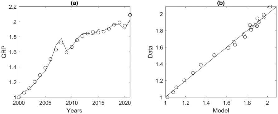
Fig. 3. Correspondence of PF (1) when using fixed capital investment as capital (C = IFC) to the initial data for 2000– 2021. (a) circles — actual GRP data, black line — model values calculated using formula (1) for A = 1, p = 0.52, q = 1.4 (Table 2). (b) circles — actual GRP data, black line — best-fit line. Adjusted coefficient of determination Ra ² = 0.99.

Nenets Autonomous Okrug. Estimates of the model parameters for the Nenets Autonomous Okrug (Table 3) show that PF (1) both with C = FAV and with C = IFC have insignificant parameters А and p , which should be excluded, i.e. log( A ) = 0 ( A =1), p = 0. The resulting model Y = L^q was also studied and, according to the estimates of its parameters (Table 3), the GRP of the Nenets Autonomous Okrug is expected to increase by 2.44% in case of NE growth by 1%. This model fits the initial data for the Nenets Autonomous Okrug better than the others (it has the minimum AICc value at significant parameters). The corresponding illustration is given in Fig. 4.

Table 3

Estimates of the model parameters for the Nenets Autonomous Okrug based on data for 2000–2021 using the value of fixed assets (C = FAV) and investments in fixed assets (C = IFC) as capital (C) 3

Parameter	Estimation	σ	t-value	Pr(>|t|)	F	p-value	R2	AICc
PF (1), С = FAV					98.3	9.5E-11	0.90	-30.9
log( A )	0.00	0.08	-0.04	9.7E-01
p	0.05	0.07	0.78	4.4E-01
q	2.26	0.37	6.06	7.9E-06
PF (1), С = IFC					95.7	1.2E-10	0.90	-30.4
log( A )	-0.03	0.07	-0.35	7.3E-01
p	-0.03	0.08	-0.37	7.1E-01
q	2.62	0.33	7.83	2.3E-07
PF (2), C = FAV					29.9	2.4E-05	0.58	-19.3

3 Column designations are given in the note to Table 2. The models that have only significant parameters and explain at least 60% of the initial data variation are highlighted in bold.

log( A )	0.27	0.05	5.05	6.1E-05
p	0.29	0.05	5.47	2.4E-05
PF (2), C = IFC					13.0	1.8E-03	0.36	-10.2
log( A )	0.16	0.10	1.58	1.3E-01
p	0.32	0.09	3.61	1.8E-03
PF: Y = Lq					195.3	4.2E-12	0.90	-35.1
q	2.44	0.06	41.06	1.5E-21
PF: Y = ACp , C = FAV					57.3	2.7E-07	0.73	-9.9
log( A )	0.37	0.08	4.92	8.2E-05
p	0.41	0.05	7.57	2.7E-07
PF: Y = Cp , C = IFC					44.8	1.3E-06	0.68	-2.5
p	0.60	0.03	19.15	8.9E-15

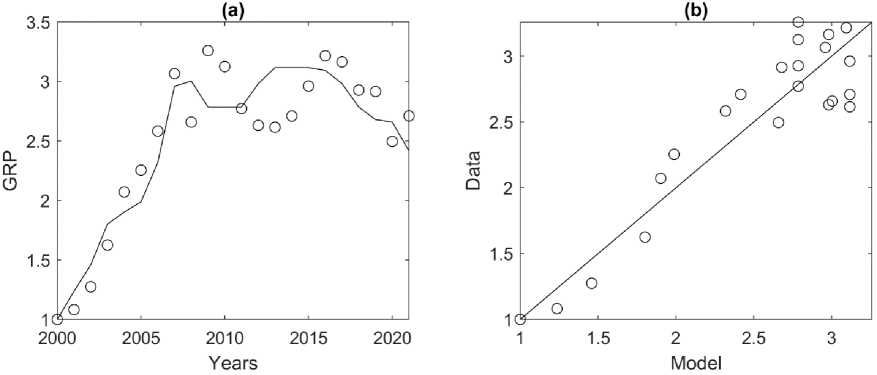
Fig. 4. Correspondence of PF Y = L^q to the initial data of the Nenets Autonomous Okrug for 2000–2021. (a) circles — actual GRP data, black line — model values calculated using formula (1) with q = 2.44 (Table 2). (b) circles — actual GRP data, black line — best-fit line. Adjusted coefficient of determination Ra ² = 0.9.

Although statistically significant (Table 3), the models in the form of PF (2) with C = FAV and C = IFC for the Nenets Autonomous Okrug) describe only 58% and 36% of the initial data variation (( Ra ² = 0.58, Ra ² = 0.36) respectively) and are therefore excluded from the analysis. In order to determine the influence of FAV on GRP, the PF model was estimated: Y = AC^p with C = FAV, which turned out to be statistically significant and explains 73% of the initial data variation (Table 3). This model has elasticity by FAV p = 0.41, therefore, if this factor increases by 1%, the expected increase in GRP is 0.41%. The model Y = C^p with C = IFC was also estimated (Table 3). This model is significant and explains 68% of the initial data variation (in the Y = AC^p model, parameter A turned out to be insignificant); estimate p = 0.60, i.e. an increase in the IFC by 1% will give an increase in GRP by 60%.

Yamalo-Nenets Autonomous Okrug. Estimates of the models for the Yamalo-Nenets Autonomous Okrug (Table 4) show that the PF (1) both for C = FAV and for C = IFC have insignificant parameters А and p, which should be excluded, i.e. log(A) = 0 (A =1), p = 0. The resulting model Y = Lq was also studied and, according to the estimates of its parameters, a 1% increase in the NE is ex- pected to increase the GRP of the Nenets Autonomous Okrug by 2.65%. This model fits the initial data for the Yamalo-Nenets Autonomous Okrug better than others (it has the minimum AICc value with a significant parameter). The corresponding illustration is given in Fig. 5.

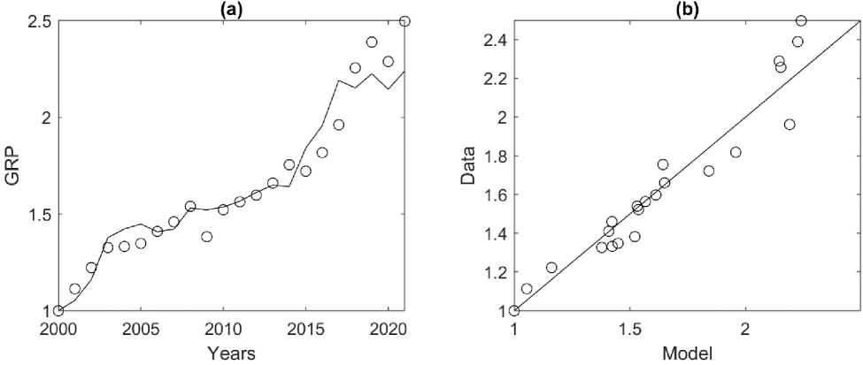
Fig. 5. Correspondence of PF Y = L^q to the initial data of the Nenets Autonomous Okrug for 2000–2021. (a) circles — actual GRP data, black line — model values calculated using formula (1) with q = 2.65 (Table 2). (b) circles — actual GRP data, black line — best-fit line. Adjusted coefficient of determination Ra ² = 0.94.

Table 4

Estimates of the model parameters for the Yamalo-Nenets Autonomous Okrug based on data for 2000–2021 using the value of fixed assets (C = FAV) and investments in fixed assets (C = IFC) as capital (C) 4

Parameter	Estimation	σ	t -value	Pr(>|t|)	F	p -value	Ra 2	AICc
PF (1), С = FAV					169.0	7.9E-13	0.94	- 57.9
log( A )	-0.07	0.05	-1.52	1.5E-01
p	0.14	0.09	1.65	1.2E-01
q	2.26	0.30	7.46	4.6E-07
PF (1), С = IFC					160.0	1.3E-12	0.94	- 56.7
log( A )	-0.01	0.03	-0.36	7.2E-01
p	0.10	0.08	1.27	2.2E-01
q	2.34	0.31	7.51	4.2E-07
PF (2), C = FAV					35.7	7.7E-06	0.62	- 37.0
log( A )	-0.16	0.08	-2.01	5.8E-02
p	0.54	0.09	5.97	7.7E-06
PF (2), C = IFC					34.1	1.0E-05	0.61	- 36.4
log( A )	0.08	0.04	1.97	6.3E-02
p	0.48	0.08	5.84	1.0E-05
PF: Y = L ^ q					312.8	4.3E-14	0.94	-60.0
q	2.65	0.07	40.627	1.9E-21
PF (2): A = 1, C = FAV					14.5	1.0E-03	0.57	- 35.4

• ⁴ Column designations are given in the note to Table 2. The models that have only significant parameters and explain at least 60% of the initial data variation are highlighted in bold.

  p	0.36	0.03	13.978	4.2E-12
  PF (2): A = 1, C = IFC					50.8	5.0E-07	0.56	- 34.9
  p	0.62	0.05	13.81	5.3E-12	14.5	1.0E-03
  PF: Y = ACp , C = FAV					75.6	3.1E-08	0.78	- 30.5
  log( A )	-0.23	0.08	-2.78	1.2E-02
  p	0.70	0.08	8.6975	3.1E-08
  PF: Y = Cp , C = IFC					89.0	5.3E-09	0.81	- 29.2
  p	0.74	0.04	19.80	4.6E-15

Models in the form of PF (2) with C = FAV and C = IFC for the Yamalo-Nenets Autonomous Okrug, although statistically significant (Table 4), have an insignificant parameter A ( Pr (>| t |) > 0.05), which should be excluded. The PF (2) estimates were made for A = 1 C = SOF and C = IFC, it turned out that they explain less than 60% of the initial data variation (Table 4), so they will not be used in further analysis.

The GRP-FAV and GRP-IFC correlation coefficients for the Yamalo-Nenets Autonomous Okrug are greater than 0.8 (Table 1), which gives us a reason to estimate separately the dependence of GRP on FAV and IFC without taking into account NE, i.e. to put q = 1 in PF (1). Then Y = AC^p , where capital C = FAV or C = IFC. The corresponding estimates are given in Table 4 in the last two lines (with C = IFC, parameter A turned out to be insignificant and was excluded). Both models turned out to be significant and describe 78 and 81% of the initial data variation, respectively. The obtained FAV elasticity value (IFC) p = 0.7 ( p = 0.74) shows that with an increase in this factor by 1%, the GRP growth is expected to be 70% (74%). Despite the fact that it was not possible to build a model of GRP production in the Yamalo-Nenets Autonomous Okrug that would include both labor and capital, the value of the IFC-NE correlation coefficient of 0.89 (Table 1) makes it possible to estimate the dependence of NE on FAV and IFC, which is given below.

Republic of Sakha (Yakutia). Estimates of the models for the Sakha Republic (Yakutia) (Table 5) show that PF (1) both for C = FAV and for C = IFC have insignificant parameters A and p, which should be excluded to avoid bias in elasticity estimates, i.e. log( A ) = 0 ( A =1), p = 0. The resulting model Y = L^q was also studied. According to estimates (Table 5), the model explains 74% of the initial data variation, and if NE grows by 1%, the GRP of Nenets AO is expected to increase by 7.49%.

Table 5 Estimates of the model parameters for the Sakha Republic (Yakutia) based on data for 2000–2021 using the value of fixed assets (C = FAV) and investments in fixed assets (C = IFC) as capital (C) 5

Parameter	Estimation	σ	t -value	Pr (>| t |)	F	p -value	Ra 2	AICc
PF (1), С = FAV					39.5	1.7E-07	0.79	-37.6
log( A )	0.01	0.06	0.21	8.4E-01
p	0.14	0.09	1.52	1.4E-01

5 Column designations are given in the note to Table 2. The models that have only significant parameters and explain at least 60% of the initial data variation are highlighted in bold.

q	6.69	1.40	4.79	1.3E-04
PF (1), С = IFC					58.1	5.8E+01	0.85	-44.6
log( A )	-0.03	0.04	-0.77	4.5E-01
p	0.24	0.08	3.22	4.5E-03
q	2.91	1.84	1.58	1.3E-01
PF (2), C = FAV					22.2	1.4E-04	0.50	-24.9
log( A )	0.26	0.03	9.26	1.1E-08
p	0.42	0.09	4.71	1.3E-04
PF (2), C = IFC					88.5	8.8E-09	0.81	-45.7
log( A )	-0.01	0.04	-0.20	8.4E-01
p	0.33	0.03	9.41	8.8E-09
PF: Y = Lq					60.0	1.4E-07	0.74	-39.3
q	7.49	0.399	18.80	1.3E-14
PF: Y = Cp , C = IFC					110.6	8.0E-10	0.84	-47.0
p	0.35	0.02	22.59	3.3E-16
PF: Y = ACp , C = FAV					26.7	4.7E-05	0.55	-22.8
log( A )	0.29	0.03	9.22	1.2E-08
p	0.46	0.09	5.17	4.7E-05
PF (2), A = 1, C = IFC					89.3	5.2E-09	0.82	-48.1
p	0.32	0.02	20.12	3.3E-15

PF (2) at C = FAV, although significant, explains only 50% of the initial data variation and is therefore excluded from further analysis. PF (2) with C = IFC has an insignificant parameter A. The estimate of this model with A = 1 shows that the model is statistically significant, explains 82% of the initial data variation and has the lowest Akaike criterion value AICc = -48.1 (Table 5) and, therefore, is the most preferable for the Sakha Republic (Yakutia). Estimates of the parameters of this model show that the contribution to GRP production by IFC is 32% (p = 0.32), and NE — 68% ( q = 1 — p = 0.68). The correspondence of this model to the initial data is shown in Fig. 6.

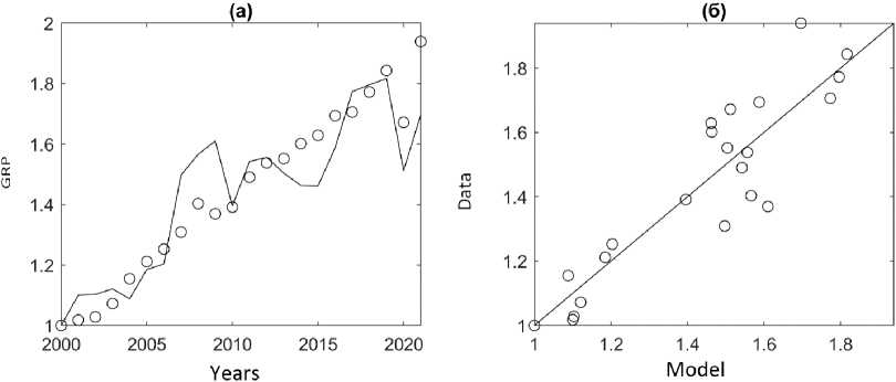
Fig. 6. Correspondence of PF (2) with C = IFC to the initial data of the Republic of Sakha (Yakutia) for 2000–2021. (a) circles — actual GRP data, black line — model values calculated using formula (2) with A = 1 and p = 0.32 (Table 2). (b) circles — actual GRP data, black line — best-fit line. Adjusted coefficient of determination Ra ² = 0.82.

The influence of capital on the production of GRP of the Republic of Sakha (Yakutia) can be quantitatively characterized using the model Y = C^p , with C = FAV or with C = IFC (Table 5). At C =

FAV, it turned out that this model explains only 55% of the initial data and cannot be used for analysis. At C = IFC (the model is significant and explains 84% of the initial data variation), it is expected that an increase in IFC by 1% will be accompanied by an increase in GRP by 35% ( p = 0.35).

Let us consider the modeling results for the regions of group 2. For these regions, constructing a model in the form of PF (1) does not make sense, since the elasticity of one of the production factors will be either statistically insignificant or even negative. The latter contradicts economic theory. Constructing a model in the form of PF (2), on the contrary, is justified and allows estimating the contribution of each factor to production. Indeed, PF (2) can be rewritten as Y / L = A ( C / L ) ^p . Let GRP-FAV correlation be positive and GRP-NE correlation be negative (e.g., the Arkhangelsk Oblast). Then the correlation of the ratios Y/L (GRP per worker) and C/L (FAV per worker) may be positive. In this case, p characterizes the contribution of FAV to GRP production, and q = 1- p is the contribution of NE to GRP production. The more NE decreases against the background of GRP growth, the higher is the Y/L ratio and the stronger is the contribution of this factor.

Arkhangelsk Oblast. Estimates of PF (2) parameters at C = FAV show (Table 6) that the model is statistically significant (p-value < 0.05) and explains 80% of the initial data variation ( Ra ² = 0.8). The contribution of FAV to GRP production is p = = 98%, and NE is q = 1 — p = 2%. In fact, the GRP of this region does not depend on the existing NE, since in 2000–2021 the NE was constantly decreasing against the background of constant growth of GRP (Fig. 2). Estimates of the PF parameters (2) with C = IFC and A = 1 (the estimate of the parameter A is statistically insignificant) show (Table 6) that the model is statistically significant and explains 66% of the initial data variation. In this two-factor model, the contribution of IFC to the production of GRP is p = = 57%, and NZ is q = 1 — p = 43%.

Table 6 Estimates of the model parameters for the Arkhangelsk Oblast based on data for 2000–2021 using the value of fixed assets (C = FAV) and investments in fixed assets (C = IFC) as capital (C) 6

Parameter	Estimation	σ	t -value	Pr (>| t |)	F	p -value	Ra 2	AICc
PF (2), С = FAV					84.1	1.3E-08	0.80	-20.5
log( A )	0.27	0.05	5.75	1.3E-05
p	0.98	0.11	9.17	1.3E-08
PF (2), A = 1, С = IFC					35.8	6.1E-06	0.66	-10.2
p	0.57	0.04	15.98	3.2E-13
PF: Y = A Cp , C = FAV					54.7	3.8E-07	0.72	-20.7
log( A )	0.28	0.05	5.62	1.7E-05
p	0.95	0.128	7.40	3.8E-07
PF: Y = Cp , C = IFC					41.8	2.1E-06	0.65	-16.9
p	0.55	0.03	17.57	4.9E-14

In order to quantitatively characterize the dependence of GRP on FAV and IFC, one-factor models (3) were estimated. According to estimates (Table 6), when SOF changes by 1% of GRP, the expected change in GRP will be p = 0.95%, and the corresponding model (Y ~ Cp) is significant and explains 72% of the initial data variation, according to the value of the Akaike criterion AICc, the model is the best for the Arkhangelsk Oblast (Fig. 7). In case of a change in the IFC by 1%, the expected change in GRP will be p = 0.55%, the corresponding model (Y ~ Cp) is significant and explains 65% of the initial data variation. It is noteworthy that there is no correlation between FAV and IFC (Table 1) for the Arkhangelsk Oblast. This explains such different values of elasticities (p) for FAV and IFC.

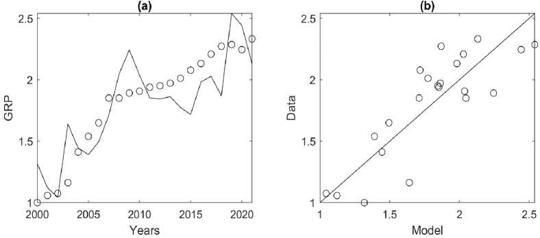
Fig. 7. Correspondence of the Y ~ C^p model with C = FAV to the initial data of the Arkhangelsk Oblast for 2000–2021. (a) circles — actual GRP data, black line — model values calculated using formula (3) with A = 1.32 and p = 0.95 (Table 2).

(b) circles — actual GRP data, black line — best-fit line. Adjusted coefficient of determination Ra ² = 0.72.

Krasnoyarsk Krai. PF (2) at C = FAV describes only 34% of the initial data variation (Table 7) and is therefore excluded from the analysis. The PF (2) assessment with C = IFC showed that the model is significant and describes 91% of the initial data variation. The contribution of IFC to GRP production is p = 33%, the contribution of NE is q = 100 — p = 67%. In this region, GRP growth occurs against the background of almost constant NE: the ratio of the maximum and minimum values for 2000–2021 is 1.06, while GRP has almost doubled during this period, and the growth of IFC has increased 5 times compared to the base year of 2000 (Fig. 2). That is, the growth of the GRP occurs due to the growth of the IFC with an actual labor shortage, therefore the contribution of the labor force to GRP is greater than the contribution of IFC.

Table 7 Estimates of the model parameters for the Krasnoyarsk Krai based on data for 2000–2021 using the value of fixed assets (C = FAV) and investments in fixed assets (C = IFC) as capital (C) 7

Parameter	Estimation	σ	t -value	Pr (>| t |)	F	p -value	Ra 2	AICc
	PF (2)	, С = FAV			11.6	2.8E-03	0.34	-12.6
log( A )	0.35	0.04	8.75	2.8E-08
p	0.64	0.19	3.40	2.8E-03
	PF (2	), C = IFC			211.0	4.3E-12	0.91	-56.4
log( A )	0.08	0.03	3.14	5.2E-03
p	0.33	0.02	14.54	4.3E-12

7 Column designations are given in the note to Table 2. The models that have only significant parameters and explain at least 60% of the initial data variation are highlighted in bold.

PF: Y = ACp , C = FAV					9.9	5.1E-03	0.30	-13.1
log( A )	0.35	0.04	8.61	3.7E-08
p	0.62	0.198	3.14	5.1E-03
PF: Y = ACp , C = IFC					228.0	2.1E-12	0.92	-59.0
log( A )	0.09	0.02	3.72	1.4E-03
p	0.32	0.02	15.10	2.1E-12

Estimates of single-factor models (3) showed (Table 7) that at C = FAV, the Y ~ C^p model explains only 30% of the initial data variation and, therefore, cannot be used in further analysis. The Y ~ C^p model at f = IFC is significant and explains 92% of the initial data variation; with a 1% change in IFC, the expected increase in GRP will be 0.32%. According to the AICc criterion values, this model best fits the original data (Fig. 8).

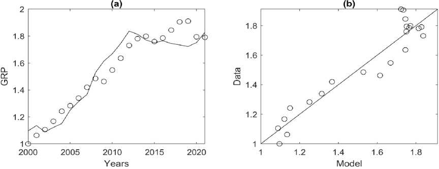
Fig. 8. Correspondence of the Y ~ C^p model with C = IFC to the initial data of the Krasnoyarsk Krai for 2000–2021. (a) circles — actual GRP data, black line — model values calculated using formula (3) with A = 1.1 and p = 0.32 (Table 7).

(b) circles — actual GRP data, black line — best-fit line. Adjusted coefficient of determination Ra ² = 0.92.

Komi Republic. PF (2) at C = FAV for the Komi Republic has Ra ² = 0.47 (Table 8), that is, the model explains 47% of the initial data variation and is excluded from the analysis. PF (2) at C = IFC is significant and explains 67% of the initial data variation; the contribution of IFC to the production of GRP p = 29%, and NE is q = 100 — p = 71%. At the same time, no significant correlation is observed between GRP and NE (GRP-NE = -0.23, GRP-IFC = 0.87, GRP-FAV = 0.18, Table 1), that is, the assessment of models of the type Y = L^q and Y = C^p at C = FAV is meaningless. The evaluation of the Y = C^p model at C = IFC shows (Table 8) that the model is significant and explains 82% of the initial data variation; if IFC increases by 1%, the expected increase in GRP will be 0.22%. This model has the minimum AICc criterion value and is the most preferable for the Komi Republic; the correspondence of this model to the initial data is shown in Fig. 9.

Table 8

Estimates of the model parameters for the Komi Republic based on data for 2000–2021 using the value of fixed assets (C = FAV) and investments in fixed assets (C = IFC) as capital (C) 8

Parameter

Estimation

σ

t -value

Pr (>| t |)

F

p -value

Ra 2

AICc

8 Column designations are given in the note to Table 2. The models that have only significant parameters and explain at least 60% of the initial data variation are highlighted in bold.

PF (2), С = FAV					19.3	2.8E-04	0.47	-33.4
log( A )	0.15	0.03	5.31	3.3E-05
p	0.30	0.07	4.39	2.8E-04
PF (2), С = IFC					44.0	1.9E-06	0.67	-44.2
log( A )	0.08	0.03	2.67	1.5E-02
p	0.29	0.04	6.63	1.9E-06
PF: Y = AC ^p, C = IFC					97.6	3.9E-09	0.82	-74.7
log( A )	0.09	0.01	6.34	3.5E-06
p	0.22	0.02	9.88	3.9E-09

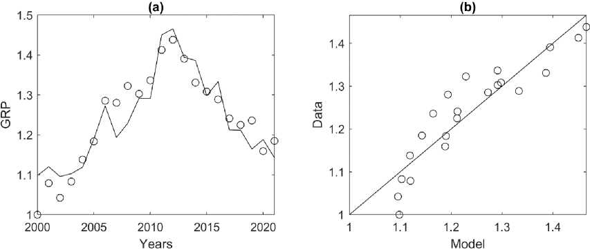
Fig. 9. Correspondence of the Y ~ C^p model with C = IFC to the initial data of the Komi Republic for 2000–2021. (a) circles — actual GRP data, black line — model values calculated using formula (3) with A = 1.09 and p = 0.22 (Table 8). (b) circles — actual GRP data, black line — best-fit line. Adjusted coefficient of determination Ra ² = 0.82.

For a number of regions (Yamalo-Nenets Autonomous Okrug, Sakha Republic, Yakutia) there is a significant correlation between IFC and NE. This allows estimating a model of the type L ~ C ^p with C = IFC and assessing the impact of the IFC on NE for these regions. The calculations show (Table 9) that for both regions the models are statistically significant and explain at least 72% of the initial data variation. For the Yamalo-Nenets Autonomous Okrug, the expected growth in NE is 0.28% with an increase in the IFC by 1%. For the Sakha Republic (Yakutia), the expected growth of the NE is 0.04% with an increase in the IFC by 1%.

Table 9 Estimates of the L ~ Cp model parameters for a number of regions of the Arctic Zone of the Russian Federation based on data for 2000–2021 using investments in fixed assets as capital (C = IFC) 9

Parameter	Estimation	σ	t -value	Pr (>| t |)	F	p -value	Ra 2
Yamalo-Nenets AO, PF: L = Cp , C = IFC					85.8	7.3E-09	0.72
p	0.28	0.01	19.41	6.8E-15
Sakha Republic		(Yakutia), PF: L = ACp , C = IFC			85.3	8.5E+01	0.80
log( A )	0.01	0.004	2.40	2.6E-02
p	0.04	0.004	9.23	1.2E-08

Conclusion

Clarification of the dynamics of GRP, investments in fixed assets, the value of fixed assets, and the number of employed in the regions of the Arctic Zone of the Russian Federation for 2000–2021 showed that there are significant differences in the production of GRP of these entities. The analysis of correlations between GRP and production factors (GRP and investments in fixed assets, GRP and the value of fixed assets, GRP and the number of employed) confirmed the initial hypothesis about the imbalance in the interaction of the main production factors in a number of regions of the Arctic Zone of the Russian Federation.

Based on the analysis of correlations, the regions of the Arctic Zone of the Russian Federation were divided into three groups: 1) regions in which the mutual behavior of the main production factors (labor and capital) fits into generally accepted concepts (the Russian Federation as a whole, the Nenets Autonomous Okrug, the Yamalo-Nenets Autonomous Okrug, the Sakha Republic (Yakutia)); 2) regions in which the mutual behavior of the main production factors does not fit into classical concepts: there is a sufficiently strong positive relationship (the square of the correlation coefficient is not less than 0.6) with only one of the production factors (Arkha n-gelsk Oblast, Krasnoyarsk Krai, the Komi Republic); 3) regions for which there is no sufficiently strong positive relationship (the square of the correlation coefficient is less than 0.6) between GRP and production factors (Murmansk Oblast, the Republic of Karelia, Chukotka Autonomous Okrug), which is only partially consistent with the previous results of modelling production processes in the regions of the Russian North and the Arctic, indicating their transformation [16, pp. 38–39].

For each region of group 1, at least 4 models were constructed in the form of PF (exponential PF and Cobb-Douglas PF were used). The best model was selected using the Akaike information criterion, adjusted for small samples. For each region of group 2, Cobb-Douglas PF models and single-factor models were estimated, which included a factor that had a positive relationship with GRP. The construction of PF models for the regions of group 3 is impossible.