Edge detection based on ant colony optimization using adaptive thresholding technique

Published Online July 2018 in MECS DOI: 10.5815/ijigsp.2018.07.07

Edge detection process could be defined as the technique of extracting the edges in a digital image. It is a set of arrangements of actions with the main purpose of identifying points in an image where variations or discontinuities in intensity take place. This set of action is vital to comprehend the substance of an image [1] and with the help of these extracted edge points. A comparison of numerous methods of image edge detection of Gradient and Laplacian based edge detection was proposed by Raman Maini and Dr. Himanshu Aggarwal [2]. Algorithms that are gradient-based like Prewitt filter have a noteworthy disadvantage of being quite delicate to noise. The size and coefficients of kernel are certain and can’t be adjusted to a given image. Thus, there is a need of an adaptive edge detection algorithm to give a robust solution that can make the adjustments as per the changing levels of noise levels these images to assist in recognizing contents of valid image from visual artifacts presented by noise.

Edge detection in Blurred images was carried out by Shweta Aggarwal by making use of Ant Colony Optimization Methodology [3]. She accomplished this edge detection in blurred digital images by giving them priority with the help of various magnitudes of color as per their quality and significance. At this point, algorithm don’t consider de-blurring of image therefore with the elimination of any chances of loss of data and a number of edges will be produced by a blur image in an area of concern is some of these edges will be of not much significance.

At this point, outcomes depend on various parameter values maintaining the level of investigation of the ants. When we enhance the value of the parameter, we get smoother edges. It must be kept in mind that this value should not be equal to, 0 and 1 but must lie in between due to the reason that it will result in loss of certain important features [4-6].

• II.    Related Work

In this section, various work performed in edge detection is detailed. This section is further divided into two sub-sections, in the first sub-section kernel based methods are discussed and in the second sub-section soft computing based methods are detailed.

• A.    Kernel Based Methods

A major portion of edge detection methodologies like Sobel, Prewitt and Robert works on the basis of gradient value. The assessed gradient pixel value in these algorithms is more than a threshold is considered as an edge pixel. Due to the fact that the threshold value is now and then empirically calculated, there is possibility that we may lose certain edges or over estimation takes place. Due to the exchange between detection and location of edge pixels, we have a problematic inaccuracy [7]. By making changes in the threshold values, the rate of edge detection enhances, still the accuracy of edge locating goes down.

Edward. et al. [8] has suggested a sub-pixel procedure for finding edges of an object which enhance the accuracy of measurement rapidly. We generally requires the sub-pixel edge detection technique and localization tools in the noisy images for the artificial vision applications, predominantly for having on line dimensional control of developed components. Various edge detection methodologies with the pixel resolution are quietly well known and a portion of them are developed to be vigorous against image corruption.

Xin et al. (2012) proposed an algorithm which is a sophisticated version of the canny edge detection algorithm that operates on color images [6]. This algorithm is based on quaternion weighted average filter (QWAF) and vector analysis to deal with the weak point of the conventional canny edge detection algorithm. The algorithm used QWAF with a sliding window of 9x9 to suppress the Gaussian noise present in the image and non-maximum suppression (NMS) which is based on interpolation for edge thinning. The Sobel operator is used to estimate the gradient of the image. The overall concert of the algorithm is very much depended on the size of the sliding window. This leads to additional blurring and thicker edges. The outline of wrecked and false edges reduces using this algorithm but the computation time is more due to the sliding window.

Gupta and Mazumdar (2013) proposed an extension of the sobel edge detection algorithm for image edge detection process [9]. The sobel edge detection method considers a 3x3 convolution kernel on an image. These kernels are extended to a 5x5 convolution kernel. Yet, the gradient approximation it produces is inaccurate. Thus, false, wrecked and thick edges exist in the output image.

Katiyar and Arun (2014) proposed a comparative analysis of common edge detection technique [10]. The comparison made between the existing edge detection algorithms such as the Sobel, Prewitt, Canny and The Laplacian. It was found that the performance of canny edge detection algorithm is better than other method with lesser number of detected false edges. However, false and wrecked edges cannot be suppressed using these techniques.

K. K. Jena (2015) investigated an edge detection method that computes image edges using the concept of Center of Mass with Sobel Operator (COM-SOBEL) [11]. This method can be used as template for multi-scale image edge detectors. They also compare the proposed method with conventional Sobel operator.

J. J. Hwang and T.L. Liu (2015) they consider contour detection using per-pixel classifications of edge point. To make possible process, a convolutional neural network (CNNs) is used to extract an instructive feature vector for every pixel and uses an SVM classifier to complete contour detection [12].

• B.    Soft Computing Approaches

We generally use three different soft computing methodologies for detecting edges for image segmentation. These three methodologies are as follows (1) Fuzzy based Approach [13], (2) Genetic Algorithm based approach [14] and (3) Neural Network based Approach [15]. These are explained underneath:

• 1.    Fuzzy based Approach

• 2.    Genetic Algorithm Approach

• 3.    Neural Network Approach

We have a number of possibilities for the development of edge detections based on fuzzy logic [14]. One of the methods is of defining a membership function showing the edginess degree in each neighborhood [14]. We can consider it as a true fuzzy approach in the case of fuzzy concepts is too applied to make the modification in the membership values. By making use of proper fuzzy if-then rules, we can generate normal or dedicated edge detections in pre-defined neighborhoods. We can test the similarity of two regions under consideration by homogeneity in the process of segmentation.

Normally, a genetic algorithm comprises three prime processes: selection, crossover, and mutation. The process of selection makes evaluation of all elements and keeps just the perfect ones [15]. Along with these, certain less fit ones could be chosen as per a small probability [15]. The others are expelled from the present population. The crossover makes the recombination of two individuals in order to get new ones which may give improved results. Changes are induced by the mutation operator induces in a few chromosomes units. This is done in order to keep up the population diversified to the extent at the time of the optimization process [15]. The purpose of Image segmentation is of making partitions of an image into homogeneous zones. Massive measures of segmentation strategies are comprehensive in the article to segment images as per the diverse criteria like color, grey level or texture. This process is not simple and quite vital, due to the reason that the yield of an image segmentation methodology can be encouraged as contribution to higher-level processing tasks. For example model-based object recognition frameworks. As of late, researchers have researched the utilization of genetic methodologies into the image segmentation issue [15].

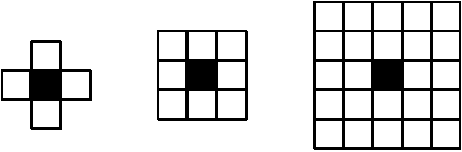
We know that neural networks are developed by numerous elements that are associated by links with different variable weights [16]. Artificial neural networks (ANN) are extensively functional for the pattern recognition [17]. Nonlinear attributes and processing potential are used for clustering. We have Kohonen Feature Map (SOFM) network as an upright tool for clustering [16]. The strategy can be detailed as follows. It comprises two free neural networks one each for intensity planes and saturation. This has three layers which are input layer, hidden layer, and output layer. In the input layer, the neuron input is harmonized between [0-1] although the output value is between [0-1]. Every layer is consisting of an exact measure of neurons equal to the size of the image. Each neuron has basic connection weight defined as 1 in [16]. Every neuron in one layer is associated to concerned neuron in the past layer with its d order neighborhood as appeared in the accompanying

Figure.1.

(a)                       (b)                           (c)

Fig.1. Neighborhoods of a pixel (a) First order neighborhood (b) Second order neighborhood (c) Sequence of neighborhood.

In the process of edge detection, begin the synaptic weights of the network, V j (0) to little, dissimilar, irregular numbers at iteration k=0. Draw a sample y from the input set. Discover the perfect matching (winning) neuron r(y) at iteration k, by making use of the least distance Euclidean criterion [16]

r ( y ) = min I | y - V j 11, j = 1,2,..., L ■

Update the synaptic weight vectors using the update formula k+1        k . k           k

V ( y ) = V r ( y ) ⁺ П ⁽ У ^- V r ( y ) )

is the neighborhood pixel of r(y). Increase k by 1 then go to the input set and then continue until the synaptic weights reach their steady-state values.

• III.    ACO Based Image Edge Detection

In this proposed technique, number of ants proceed onward a 2-D picture, venturing starting with one pixel then onto the next to build a pheromone matrix, which decide the edge data for every pixel area in the picture to separate the edges of the picture. Edge detection contains the accompanying steps as defined below [18-27]:

Initialization process

In this procedure for a picture I of size M 1 × M 2 is taken as input information which functions as an solution space for the manufactured ants. The K quantities of ants are haphazardly moved over the entire picture with the end goal that the each pixel of the picture is seen as a node. The constant is allotted to every, which is the underlying estimation of each part of the pheromone matrix. The initial value of each component of the pheromone matrix T (0) is set to be a constant.

Construction Process

One ant is irregularly chosen at the nth constructionstep from the above-discussed whole K ants, and this ant will continuously move on the image for L movement- steps. This ant moves to its neighboring node (i, j) as per the transition probability that is [22-26]

p ( l , m )( i , j )

№Г ( П _и ) ^e

X ( t- 7“ У ( n ,j )¹' i , j E ^ ₍ i , m )

In the above equation, T_t ⁽ ” 1) is defined as the pheromone value of the node ( i , j ), the parameter Ω ( l , m ) represents the neighborhood nodes of the node ( l , m ), the parameter η i , j defines the heuristic information at the node ( i , j ). The effect of the pheromone matrix and the heuristic matrix is represented by the constants α and β respectively.

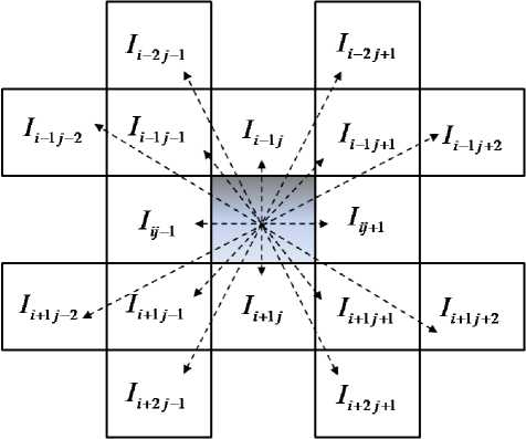
Fig.2. Representation of clique.

The procedure comprises two vital issues and these are given beneath: The main issue is the heuristic data П j which can be determined by the local insights of the picture which relies on upon inner clique c. The local statistics at the pixel area ( i , j ) is figured as takes after [27]

П . , , = | V c ( i , j )                     (2)

Now, here the parameter Z represents a normalization factor, means the capacity of a neighborhood gathering of pixels c which is called coterie [28]. Determines the power estimation of a pixel at a location ( i , j ) of a picture I and is given with the help of the below equation

Z = XX V c ( i , j )         (3)

• i = 1: M_x j = 1: M₂

The parameter Z defines a normalization factor, while I represents the measure of intensity of the pixel at the

(i, j) position of the image I, the function V (i, j) is a function of a local group of pixels (known as the clique), and its estimation relies on the changes in intensity values of image of the clique c (as illustrated in Figure 2). All the more particularly, for the pixel I under consideration, the function V (i, j)is

^V c (It , j ) = f (I 11 - 2, j - 1 - I i + 2, j + 11 ⁺ | I i - 2, j + 1 - I i + 2, j - 11

• ⁺    | I i - 1, j - 2 ^- Ii + 1, j + 2 | ⁺ | I i - 1, j - 1 ^- Ii + 1, j + 11

• ⁺    | I i - 1, j ^- Ii + 1, j | ⁺ | I i - 1, j + 1 ^- Ii - 1, j - 11

• ⁺    | I i - 1, j + 2 ^- Ii - 1, j - 2 | ⁺ |Л, j - 1 ^- Ii , j + 11)

In order to find out the function f(·) in (4), the four functions mentioned below are considered in this work;

_ ( n - 1) ^T i, j

₌ \1 - p)< j 1) + P< j

" T j ¹

if ( ij ) e visited current ant otherwise

At this point, the parameter ρ represents the rate of evaporation of pheromone that relies on the measure of user choice, is estimated by the heuristic matrix.

We carry out the second update after the movement of the whole ants in each construction-step as:

т ^{( n} ) = (1 - ^ ) T ^{( n - 1)} +^t ⁽⁰⁾          (10)

f ( x ) = X x   for x >  0            (5)

f ( x ) = X x ²

^{f ( x} ) =

^{f ( x} ) = •

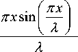
sin

for x >  0

0 < x < X otherwise

0 <  x <  X

otherwise

The parameter λ defined in the functions (5)-(8) modifies the functions’ respective shapes. The second problem is to find out the acceptable range of the ant’s movement (i.e., Ω (l,m) in (1)) at the position ( l , m ). In this paper, it is considered to be 8-connectivity neighborhood, as demonstrated in Fig 3.

Now, the parameter ψ represent the pheromone decay coefficient expands the look for the consequent ants by diminishing the pheromone level on the traversed edges. Along these lines it gives a chance to the consequent ants to create fundamental arrangements. Consequently, the probability of reiteration turns out to be more improbable in a similar iteration [29].

Decision process

In this progression, a binary decision is made at each pixel location to find out whether it is edge or not, by making application a threshold T on the last pheromone matrix τ ^(N) . We propose the above-discussed T in this research article to be adaptively estimated on the basis of the technique created in [30]

We choose the initial threshold T^{( 0)} as the pheromone matrix mean value. After this, the entries of the pheromone matrix is ordered into two classifications as per the standard that its value is not more than T^{( 0)} or bigger than T^{( 0)} . At that point the latest threshold is registered as the average of two mean values of all of the above two classes. The discussed procedure is rehashed till the point the threshold value doesn’t vary any more (as far as a user- characterized tolerance). We can define the above iterative technique as.

Step 1: Initialize initial threshold T^{( 0)} as

Fig.3. 8-connectivity neighborhood.

у У    T N )

гр (0) _ ^-^ i = 1: M ] X—l j = 1: M ₂   ⁱ , ^j

MM

And consider iteration value as q = 0.

Step 2: Make the separation of the pheromone matrix T ⁽ N ) into two class making use of T ⁽ l ) , here the first class comprises entries of τ that have not more values than T ^{( l )} , on the other hand the second class comprises the left over entries of τ. After this, make the calculation of the mean of all of the above two classes through

Update Process

In the update process, we update the pheromone matrix after the two operations of updation. The initial update is performed after the mobility of every ant in every development step. Every block of building of pheromone matrix is altered as provided in equation (9):

У У g^L T N )

(l)    iL-^i=1: M,Z—ij =1: M2°T(1)  i,j mL У У hL T(N)

^ i = 1: M 1 ^ j = 1: M ₂ TT ⁽ ' ) ^il , ^j

Where,

mu =

U ( N ) ₂ g_T ( l ) i , j

U ( N )

t 2 h T ⁽ ')^Ti , j

PSNR — 10 log-55- MSE

MSE = mean square error; This is given as:

L	x	x <  T ( l )
g T ( 1 ) — ’	[ 0	otherwise
h L i ) —	I 1	x <  T ( l )
	[ 0	otherwise
и	x	x >  T ( l )
gT( l ) —	[ 0	otherwise
h U ) — <	'1 0	x >  T ( l ) otherwise

MSE — [ I g ( i , j ) — 1 ₀( i , j )] 2             (23)

In above I ( i , j ) is ground truth image and I ( i , j ) is image obtained through Sobel, Canny and ACO methods.

Berkeley Segmentation Dataset (BSD) Images

Step 3: Set the iteration index q = q + 1, and select new threshold as

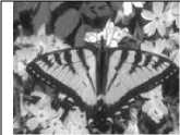
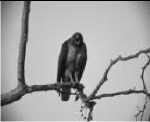
Image No. 42049

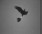
Image No. 135069

T ( l )

m(L1) + m (l)

Step 4: In the case of | T ^l — T ^l 1) >  £ , then go to Step 2 ; else, the iteration method is terminated and make a binary decision on each pixel position ( i , j ) as an edge as

E i,j

—I1

( N )        ( l )

i,j otherwise

In the simulation BSD (Berkeley Segmentation Dataset) is considered. Here, six images are considered, where both RGB and ground truth edge images are obtained. The performance evaluation is measured in terms of Peak Signal to Noise Ratio (PSNR), Performance Ratio (PR) and Efficiency (EF). The performance ratio (PR) is defined as:

True Edges                ₍₂₀₎

False Edges

The efficiency (EF) is defined as:

True Edges

EF —

True Edges + False Edges

The well-known peak-signal-to noise ratio (PSNR) is defined as:

Image No. 118035

Image No. 189011

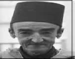
Image No. 189080

The Berkeley Segmentation Dataset (BSD) images [31] and respective ground truths are used in this simulation. This dataset is comprehensive but some of the images are more frequently used in edge detection process. We considered the same images for the simulation experiments. In total we have considered six images along with the ground truth images which contain ideal edges.

The obtained edge detected image will be compared with ground truth image and results will be compared in terms of PSNR, PR and EF as defined above.

The simulation parameters for ACO are detailed below:

• •    K = ^ JMM j : the total number of ants used for edge detection.

• •    T init = 0.0001: the initial value of each component of the pheromone matrix.

• •    a = 1: the weighting factor of the pheromone

information.

• •    в = 0.1: the weighting factor of the heuristic

information.

• •    Q = 8-connectivity neighborhood: the permissible ant’s movement.

• •    X = 10: the adjusting factor of the functions.

• •    p = 0.1: the evaporation rate.

• •    L = 40: total number of ant’s movement-steps within each construction-step.

• •    v = 0.05: the pheromone decay coefficient.

• •    ε = 0.1: the user-defined tolerance value used in the decision process of the proposed method.

• •    N = 4: total number of construction-steps.

In Figure 4, results for one BSD image are shown. In figure (a) image under consideration is shown. In figure (b) ground-truth image is shown. Canny edge detection is shown in figure(c), detected image using Sobel detection is shown in figure (d). The performance of canny and Sobel is nearly similar. But the performance of canny detection is slightly better. But in both the methods number of falsely detected edges are large in number. In figure (e) to (h) results for ACO are shown and images (e) and (g) are similar and close to ground truth image, however it fail to detect some of the true edges, but it does not accept false edges.

(a)Original Image	(b) Ground truth
(c) Canny Edge	(d) Sobel Edge
	/ <
(e) Edge detected ( f 1)	(f) Edge detected ( f 2)
	\           7
	1 (
X       Z. -
(g) Edge detected ( f 3)	(h) Edge detected ( f 4)

Fig.4. (a) Original image (b) ground truth (c) Canny Edge (d) Sobel Edge (e) Edge detected ( f 1 ) (f) Edge detected ( f 2 ) (g) Edge detected ( f 3 ) (h) Edge detected ( f 4 )

By visualizing the images it is not possible to distinguish among them, therefore parameters PSNR, PR and efficiency are considered to compare them. The obtained results are shown in Table 1.

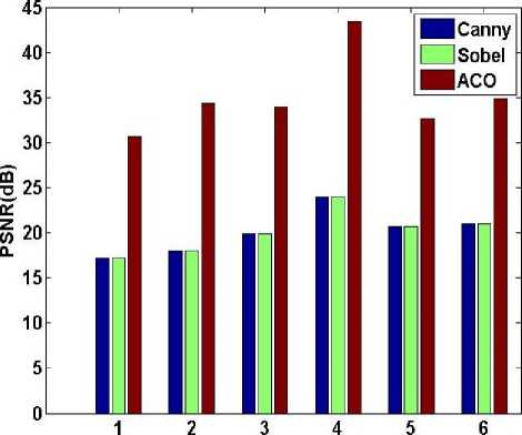
The PSNR values for proposed method are much larger than Canny and Sobel methods. For all the considered images a significant improvement is observed in PSNR values. It is also notable that the PSNR value is relative to the ground truth image and if edge detected image is exactly similar to ground truth image then PSNR is infinite. Thus higher values of PSNR also measure of similarity between the compared results. More PSNR means more similarity. It can also be visualized that in figures that edge detected image using proposed method is very much similar to ground truth image. Thus a relatively higher PSNR is obtained. In past the obtained PSNR is nearly 17 dB which represents a very poor quality of image. However with ACO the obtained PSNR is greater than 30dB, which is of good quality. Relatively higher value of PR also indicates that more true edges are found in comparison to false edges. Efficiency clearly indicates that in this method a minimum of nearly 88% edges are correctly identified, with a maximum of nearly 97.5%.

Table 1. Comparison of vital parameters with various test functions

Functions	PSNR (dB)	PR	Efficiency
Image Number : 35010
f 1	31.01643	724.16965	87.86658
f 2	30.75868	971.69435	90.66898
f 3	30.96751	780.88476	88.64778
f 4	30.71215	991.27199	90.83638
Image Number : 42049
f 1	34.86384	1181.09611	92.19418
f 2	34.32998	1534.14387	93.88059
f 3	34.86921	1131.22137	91.87798
f 4	34.48011	1455.35198	93.57059
Image Number : 135069
f 1	34.46126	1068.76812	91.44398
f 2	34.06315	1564.49948	93.99219
f 3	34.52012	1051.24911	91.31378
f 4	33.97681	1630.57940	94.22159
Image Number : 118035
f 1	45.02702	3007.70713	96.78219
f 2	43.44985	3777.16346	97.42079
f 3	45.48155	2897.95539	96.66439
f 4	43.62238	3695.05882	97.36499
Image Number : 189011
f 1	33.12695	1455.35198	93.57059
f 2	32.65058	2493.08682	96.14359
f 3	33.08451	1501.68818	93.75659
f 4	32.65652	2448.02528	96.07539
Image Number : 189080
f 1	35.38420	1574.87020	94.02939
f 2	34.90836	2452.05696	96.08159
f 3	35.39088	1587.13389	94.07279
f 4	34.92551	2366.20795	95.94519

Images

Fig.5. PSNR vs. images for Sobel, Canny and ACO

using ACO is more than 30 dB, thus the obtained edge detected images are of good quality, as in previous work PSNR was below 20 dB, and for such low PSNR images can’t be used for further processing.

In Fig.6, for all the considered six images PR is plotted. Again for ACO PR is very high. Thus, the false edges are very lesser in ACO methods in comparison to other two methods.

In Fig.7, for all the considered six images efficiency is plotted. Here for ACO efficiency ranges from 88 to 97.5%. Thus, the overall efficiency is very good; it clearly shows that large numbers of true edges are detected.

• VI. Conclusions

  

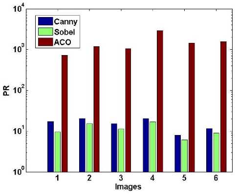
  Fig.6. PR vs. images for Sobel, Canny and ACO

  
  

Edge detection process is an important part of image processing. It is found applications in many areas of research in the field of computer vision and image segmentation. Edge detection provides important information like feature detection etc. The success of edge detection depends on the technique and optimal threshold. This paper discusses the implementation of a technique for image edge detection based on Ant Colony Optimization (ACO). It considers the various advantage of ant colony like stigmergy, distributed computation, pheromone evaporation, decision-making based on pseudo-random proportional rule. These features are very much beneficial for the determination of pheromone matrix, which contains information related to the edge. Therefore, over decades lots of techniques are investigated and developed for the correct detection of edge. ACO is a method based on heuristic search and it is beneficial for discrete problems. An ACO algorithm for image edge detection has been investigated. Here for ACO efficiency ranges from 88 to 97.5%. Thus, the overall efficiency is very good; it clearly shows that large numbers of true edges are detected.

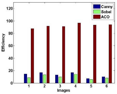
Fig.7. Efficiency vs. images for Sobel, Canny and ACO

• [1]    R. Gonzalez and R. Woods, “Digital Image Processing,” Addison Wesley, 1992, pp 414 - 428.

• [2]    Maini, Raman, and Himanshu Aggarwal. "Study and comparison of various image edge detection techniques." International journal of image processing (IJIP) 3.1 (2009): 1-11.

• [3]    Jaiswal, Utkarsh, and Shweta Aggarwal. "Ant colony optimization." International Journal of Scientific and Engineering Research 2.7 (2011): 1-7.

• [4]    Vasavada J, Tiwari S. “A Hybrid Method for Detection of Edges in Grayscale Images.” International Journal of Image, Graphics and Signal Processing. 2013 Jul 1; 5(9):21.

• [5]    Mamoria P, Raj D. An Analysis of Fuzzy and Spatial Methods for Edge Detection. International Journal of Information Engineering & Electronic Business. 2016 Nov 1; 8(6).

  In Fig.5, for all the considered six images PSNR is plotted. It is clear from the figure that the PSNR for ACO much more superior to other two methods. The PSNR

  
  

• [6]    Xin G., Ke C., and Xiaoguag H. (2012). An improved Canny edge detection algorithm for color image. Institute of Electrical and Electronics Engineers Transcations , pp.113-117.

• [7]    Wang, Rong, et al. "An edge detection method by combining fuzzy logic and neural network." Machine Learning and Cybernetics, 2005. Proceedings of 2005 International Conference on . Vol. 7. IEEE, 2005.

• [8]    Lyvers, Edward P., et al. "Subpixel measurements using a moment-based edge operator." IEEE Transactions on pattern analysis and machine intelligence 11.12 (1989): 1293-1309.

• [9]    Gupta S., & Mazumdar S. G. (2013). Sobel edge detection algorithm. International journal of computer science and management Research, 2 (2), pp.1578-1583.

• [10]    Katiyar, & Arun. (2014). Comparative analysis of common edge detection techniques in context of object extraction. IEEE Transactions of Geoscience and Remote Sensing, 50 (11), pp.68-79.

• [11]    Jena, Kalyan Kumar. "Application of COM-SOBEL operator for edge detection of images." IJISET, Engineering & Technology 2.4 (2015): 48-51.

• [12]    J.-J. Hwang and T.-L. Liu. Pixel-wise deep learning for contour detection. In ICLR, 2015.

• [13]    Om Prakash Verma et. al., “A Novel Fuzzy Ant System for Edge Detection”, in Proc. of the 9th IEEE International Conference on Computer and Information Science, pp.228-233, 2010.

• [14]    Stutzle and H. Holger H, “Max-Min ant system,” Future Generation Computer Systems , vol. 16, pp. 889–914, Jun. 2000

• [15]    Jin-Yu, Zhang, Chen Yan, and Huang Xian-Xiang. "Edge detection of images based on improved Sobel operator and genetic algorithms." Image Analysis and Signal Processing, 2009. IASP 2009. International Conference on . IEEE, 2009.

• [16]    Srinivasan, V., P. Bhatia, and Sim Heng Ong. "Edge detection using a neural network." Pattern Recognition 27.12 (1994): 1653-1662.

• [17]    M. Dorigo, L. M. Gambardella, M. Middendorf and T. Stutzle, “Special Issue on Ant Colony Optimization”, IEEE Transactions on Evolutionary Computation, vol. 6, Jul. 2002.

• [18]    Gupta S., and Mazumdar S. G. (2013). Sobel edge detection algorithm. International journal of computer science and management Research, 2 (2), pp.1578-1583.

• [19]    D.S. Lu and C.C. Chen, “Edge detection improvement by ant colony optimization”, Pattern Recognition Letters, vol. 29, pp. 416–425, Mar.2008.

• [20]    Jing Tian, Weiyu Yu, and Shengli Xie, ”An Ant Colony Optimization Algorithm for Image Edge Detection”, in Proc. of the IEEE International, pp.751-756, 2008.

• [21]    Gupta, Charu, and Sunanda Gupta. "Edge detection of an image based on ant colony optimization technique." Int. J. Sci. Res.(IJSR) 2.6 (2013): 1256-1260.

• [22]    X. Zhuang, “Edge Feature Extraction in Digital Images with the Ant Colony System”, in proc. of the IEEE international Conference an computational intelligence for Measurement Systems and Applications , pp.133-136, 2004.

• [23]    R. Rajeswari and R. Rajesh, “A modified ant colony optimization based approach for image edge detection,” International Conference on Image Information Processing (ICIIP) , pp. 1–6, 2011.

• [24]    M. Dorigo and S. Thomas, “Ant Colony Optimization”. Cambridge: MIT Press, 2004.

• [25]    H.B. Duan, “Ant Colony Algorithms: Theory and Applications”. Beijing: Science Press, 2005.

• [26]    M. Dorigo, M. Birattari and T. Stutzle, “Ant colony optimization”, in proc. of the IEEE Computational Intelligence Magazine , pp.28.39, 2006.

• [27]    Anna Veronica Baterina and Carlos Oppus, “Image Edge Detection Using Ant Colony Optimization”, International Journal of circuits, System and Signal Processing , Issue 2 vol.4, pp. 25-33, 2010.

• [28]    J. Tian, W. Yu, and S. Xie, “An ant colony optimization algorithm for image edge detection,” in I EEE World Congress on Evolutionary Computation , pp. 751 –756, Jun. 2008.

• [29]    P. Xiao, J. Li, and J.-P. Li, “An improved ant colony optimization algorithm for image extracting,” in Apperceiving Computing and Intelligence Analysis (ICACIA) , 2010 International Conference on, pp. 248 – 252, Dec. 2010.

• [30]    N. Otsu, “A Threshold Selection Method from Gray-level Histograms,” IEEE Trans. on Systems, Man and Cybernetics , vol. 9, no. 1, pp. 62–66, 1979.

• [31]    Khaire, Pushpajit A., and Nileshsingh V. Thakur. "A fuzzy set approach for edge detection." International Journal of Image Processing (IJIP) 6.6 (2012): 403-412.