EFF-ViBE: an efficient and improved background subtraction approach based on ViBE

Автор: Elie Tagne Fute, Lionel L. Sop Deffo, Emmanuel Tonye

Журнал: International Journal of Image, Graphics and Signal Processing @ijigsp

Статья в выпуске: 2 vol.11, 2019 года.

Бесплатный доступ

Background subtraction plays an important role in intelligent video surveillance since it is one of the most used tools in motion detection. If scientific progress has enabled to develop sophisticated equipment for this task, algorithms used should be improved as well. For the past decade a background subtraction technique called ViBE is gaining the field. However, the original algorithm has two main drawbacks. The first one is ghost phenomenon which appears if the initial frame contains a moving object or in the case of a sudden change in the background situations. Secondly it fails to perform well in complicated background. This paper presents an efficient background subtraction approach based on ViBE to solve these two problems. It is based on an adaptive radius to deal with complex background, on cumulative mean and pixel counting mechanism to quickly eliminate the ghost phenomenon and to adapt to sudden change in the background model.

Еще

Background subtraction, ViBE, adaptive radius, cumulative mean, pixel counting, ghost

Короткий адрес: https://sciup.org/15016028

IDR: 15016028 | DOI: 10.5815/ijigsp.2019.02.01

Текст научной статьи EFF-ViBE: an efficient and improved background subtraction approach based on ViBE

Published Online February 2019 in MECS DOI: 10.5815/ijigsp.2019.02.01

II. Background

Naively, the basic idea behind background subtraction will just consist of the difference between the current pixel value and the background model value followed by the comparison of that difference to a threshold value for decision. However, in real life situations there is a lot of complexity in the background due to many challenges namely illumination changes, dynamic background, camera jitter and many other background challenges. This leads to the development of more sophisticated techniques for background subtraction purpose.

Probabilistic background subtraction techniques also called parametric background subtraction techniques generally refer to approaches that model the background using a Normal (Gaussian) distribution over pixel’s intensity values of an image. Many solutions exist in the literature, but one of the first was proposed by Stauffer C et al[6]. It was followed by many improved methods STGMM[9], SKMGM[10], SKMGM[10], TAPPMOG[11] and STAPPMOG[12] (where MOG stands for mixture of Gaussian) each of them trying to solve one or more insufficiency(ies) of the original algorithm. However, dues to its sensitivity, MOG approach cannot be accurately tuned and its ability to successfully handle high and low-frequency changes in the background is debatable.

To solve the drawbacks of manually selecting parameters in each environment, non-parametric approaches were proposed (Ahmed Elgamma[13]). They generally refer to sample-based methods but many other methods exist such as kernel density estimation (KDE) approach[14], the Bayesian approach[15] or recursive density estimation (RDE) approach[16].

Another family of method is codebook approach where for each pixel position, the background is modeled by a codebook. It was introduced by Kim et al[17]. Here each pixel is assign a codeword which consists of intensity, color and temporal features. To do the segmentation, the intensity and color of incoming pixels are compared with those of the codewords in the codebook. Later on, the algorithm computes the distances between the pixels and the codewords, compare them with a threshold value and assign either a foreground label if no match was found or a background label otherwise. Later on, the matching codeword is updated with the respective background pixel.

We also have subspace based approach[18], in which one model is devoted. to accurately detect motion, while the other aims to achieve a representation of the empty scene. The differences in foreground detection of the complementary models are used to identify new static regions. In this approach, a collection of images and the corresponding mean and covariance matrix are computed. This is followed by the computation of PCA of the covariance matrix, a projection with a certain number of vectors and a comparison of incoming images with their projections onto Eigen vectors. Finally a distance is computed between the image and the projection and compared with the corresponding threshold value to label the pixel as foreground or background pixel.

Moreover we have compressive sensing approaches[19, 20, 21, 22], which allow reducing the number of measurements required to represent the video using the prior knowledge of sparsity of the original signal. Its theory shows that a signal can be reconstructed from a small set of random projections, provided that the signal is sparse in some basis as an example in the case of wavelets. However these methods impose certain conditions on the design matrix.

It is also important to mention approaches that use edge detection[23], or patches detection[24]. While the first approach is used most frequently for image segmentation based on abrupt changes occurred in image intensities, the second one uses patch-based approaches for operations such as image denoising.

A more recent approach developed by Braham and Droogenbroeck is the use of convolution neural network generally refers as deep learning approach. It uses a fixed background model, which was generated from a temporal median operation over N video frames [25]. Its architecture is very similar to LeNet- 5 network for handwritten digit classification[26], except that sub sampling is performed with max-pooling instead of averaging and hidden sigmoid units are replaced with rectified linear units for faster training. However, this method tends to be scene specific that is why we will not focus on it in this paper.

This paper presents an efficient background subtraction approach based on ViBE named EFF-ViBE where EFF stands for efficient. The proposed approach has three main contributions. The first contribution is the introduction of a new update mechanism that uses Koenig formula to reduce overall computations. This is combined with the use of n recent frames to model the background. Here the value of n has been chosen empirically. The second contribution lies on the introduction of a pixel counting mechanism to consider foreground pixels that stay for long as background pixels. This usually happens when a sudden change appears in the background model. Note that these two contributions are to quickly eliminate the apparition of ghost phenomenon. Finally the third contribution concerns the introduction of a modified adaptive radius policy with parameter adjustment which enables the algorithm to deal with complex background when necessary and behave differently (almost as the original ViBE) when the background is relatively simple.

III. Vibe Algorithm

The following section describes original version of ViBE algorithm proposed by Barnich et al in^[5] as well its improvement^[27] proposed by the same authors in order to handle video sequences. Its background model is a nonparametric pixel based model where each background ground pixel x is modeled by a set of samples.

M = ( ^V 1 , v 2 , v 3 — v N } ⁽¹⁾

It follows the same structure as any background subtraction algorithm which has three sub-tasks namely background model initialization, segmentation or classification and update of the model.

A. Background Model Initialization

For each pixel x , the set M ( x ) is filled randomly with samples around the spatial neighborhood of x . It is important to mention that those values are taken in the first frame and an assumption that neighboring pixels share a similar temporal distribution is made. The background estimate is therefore valid starting from the second frame. If t = 0 indexes the first frame and that N G ( x ) is a spatial neighborhood of a pixel location x , therefore

M 0 = { v ⁰ ( yy e N G ( x ⁾ ^)} (2)

where locations y is chosen randomly according to a uniform law.

B. Classification Process

In practice, ViBE does not estimate any probability density function, but uses a set of previously observed sample values as a pixel model. If the algorithm wants to classify a value v(x) of a pixel x, it compares this value to the closest values among the set of samples by defining a sphere SR(v(x)) of radius R centered on v(x). If the intersection set of this sphere and the set of samples {v1, v2, ..., vN } is above a given radius #min, then the pixel is classified as background pixel. Mathematically, #min is compared to:

# ^{ ^S R ⁽ v ⁽ x ) ) A ^{ v i , v 2 , v 3„ . v_w ^}} (3)

C. Backgroun Model Update

To update the model, the algorithm uses three powerful techniques namely memory-less update policy, random sampling and spatial diffusion.

• Memory-less update policy

This consists in choosing randomly the sample to be updated. If the probability of a sample present in the model at time t being preserved after the update of the pixel model is given by N - ¹ it will have the value

( t + dt ) — t

P(t,t + dt)=l N--1

for any further time, t+ dt . This can be rewrite as

, (N - 1 ) „

-lnl I

P(t, t + dt) = e 1 N J

• Random sub-sampling policy

This policy decides randomly which pixels are updated. By default, the adopted time sub-sampling factor ϕ is 16 meaning that each background pixel value has 1 chance in 16 of being selected to update its pixel model

• Spatial diffusion policy

D. Other Approaches Related to Vibe

Another update mechanism consists of a first-in first-out model update policy such as those employed in^{[28, 29]}, 300 samples cover a time window of only 10 seconds (at 30 frames per second). A pixel covered by a slowly moving object for more than 10 seconds would still be included in the background model. More recent techniques such as^[30]suggest that one frame alone cannot distinguish whether pixels belong to the foreground or background. Therefore, they propose to use the first n frames of the video sequence to complete the initialization of the background model. Others such as^[31], believe that for complex dynamic background, the radius R should be increased appropriately, so that the background cannot be easily detected as foreground. On the other hand, they also believe that for simple static background, R should be decreased to detect small changes of the foreground.

IV. Description of Eff-Vibe Technique

In this section, we are going to explain in details the EFF-ViBE approach. The overall functioning can be divided as the original ViBE in three main parts namely background model initialization, background segmentation and background model update. The idea is, rather than using the first frame to initialize the N sample values of each pixel, we instead use the n first frames. This enables to take into consideration the relationship between the n recent frames and thus acts as a filter. In addition, pixel counting mechanism comes and reinforces the process, if a foreground pixel stays in the foreground during K consecutive frames; it has certainly become a background pixel since it is now a static pixel in the scene

To see the advantage in using n recent frames to model the background we can analyze Fig 1. It shows the difference in the results between the use of one frame and the use of n recent frames in comparison to the perfect waited output. We can easily see that it is better to choose the n recent frames for, the results are more accurate. The drawback of this approach is that it needs a little bit more computational resources (especially memory and time) than the one using one frame but, it is acceptable compared to the results obtained.

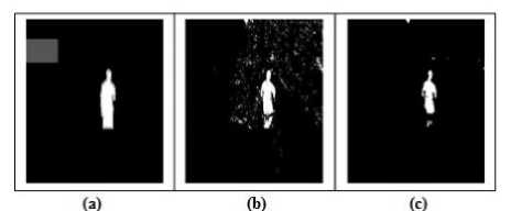
Fig.1. Comparison of the results on overpass dataset (a) the ground truth (b) the output using one frame (c) the output using n recent frames

On the other hand, when some modifications occur in the background as in the case of movement of branches, of the air, of small particles or even small waves at a sea surface, we have to handle this complexity. This is because those elements in movement do not belong to the foreground and thus must be treated as background elements. Yet, using a fix radius R can mistakenly classify those pixels as foreground pixels. That is why we use an adaptive radius (we have decided to denote it R _ad ) that tends to be steady if the mean distance between the current pixel and its N sample background values increases gradually for complex dynamic background and tends to lightly decrease if the mean distance tends to be steady.

(a) (b) (c)

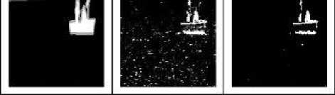
Fig.2. Comparison of the results on boats dataset (a) the ground truth (b) the output using a fixed radius (c) the output using an adaptive radius.

Fig 2 shows the difference in the results between the use of a fixed radius and the use of an adaptive radius in comparison to the perfect waited output. The drawback is still the same as the previous one so it is acceptable.

All this has enabled us to formalize the whole process schematically and it is presented on Fig 3

The proposed EFF-ViBE method has three main parts namely background initialization, background segmentation and background update as shown in Fig 3. The first part is performed during the initialization process. While the first n frames are gathered to compute the cumulative mean for each pixel, the sample values are initialized as well. At the same time, an adaptive radius R ad is also computed for each pixel. The second part is the segmentation part that classifies a pixel as background or foreground pixel if conditions in the segmentation block of Fig 3 are verified or not. The third part is performed after the segmentation process. It uses each new incoming frame to update its parameters. In this part, we try to update the parameters used with a particular approach. Since computing the mean and the standard deviation (at each iteration) for every pixel is costly, we use the fact that to compute a new mean, we only need to retrieve the first pixel's history value and add the new value on the previous mean and do the same for the standard deviation. Consequently the new mean will be function of the previous mean, the first value and the new observed value. The new standard deviation will use the same principle meaning that it will be function of the previous standard deviation, the first value and the new observed value. In addition, to compute the new adaptive radius, we also avoid computing it (at each iteration) instead we compute a new radius if and only if the history values of the corresponding pixel have changed. In a generic manner if we denote by “change” the variable that indicates if the history values of a pixel have changed or not, the update mechanism will use the history of the pixel and the “change” value to compute the new radius. The details on the method will be given in the following subsections, where the mathematical expressions are given.

A. Modified Background Model Initialization

To initialize the background model we use three techniques. Firstly, we use the initialization process of the normal ViBE method to model each background pixel with N sample values taken from their direct neighborhood. Secondly, we use the n first frames as in^[30]but with a modification of its value, for we have noticed that increasing the number of frames also increase the accuracy of the results. On the other hand, if n is too high the algorithm becomes slower. That is why we have chosen n equal to 30 instead of 20 as in the original paper. The chosen frames are used to compute the mean value of each pixel and we add this value to the sample values to have N + 1 sample values. This leads each pixel to be modeled by

M = { v ( x ) 4, v 2 , V3—V N } (6)

where

n v0 (x )=-Z V (x ) (7)

n t = 1

Thirdly we use the N sample values as in[31] to compute an adaptive radius for each pixel. We have obtained our values empirically in relation to the values chosen in the original paper. After several tests we have noticed that the original values can be modified that is S, increased a little bit and £d decreased. Consequently we have chosen S equal to 0.08 rather than 0.06 and £d equal to 0.35 rather than 0.4. We have chosen to denote the adaptive radius Rad as

N dmean = ^ ^ (X ) (9)

i = 1

Where D i ( X ) is the distance between pixel

and

sample value v i.

B. Modified Background Model Segmentation

If we denote by B the segmented image, B ( x) will be the value of the pixel x in matrix B which is equal to 0 if x is a background pixel and 255 if x is a foreground pixel. Therefore, to classify a pixel as background pixel or foreground pixel we use the following equations for:

,. .. min .. .. ^v t ⁽ ^x ^)e S T ⁽ ^v 0 ⁽ ^x )) (10)

255,......... otherwise

Г R ad , T = ^

CT = JZ(vt(X )- v0 (x ))

V t = 1

The parameter U_min will be set to 2 as in^[5,30,31], and β will be set to 3 as in^[30]. In addition, we have noticed that in the specific situation of camera jitter and thermal condition choosing a factor of 1.5 rather than 4.5 as in the original paper to update the last history of the background model leads to better results

C. Proposed Background Model Update

To update our model we use the following assumptions. Firstly, as stated in[5], we consider that neighboring background pixels share a similar temporal distribution and that a new background sample of a pixel should also update the models of neighboring pixels. For that reason, we use the same memory-less up date policy as well as the time sampling policy. This enables the sample values of each pixel to adapt to background change.

Secondly, we use a pixel counting mechanism that classifies a pixel that stays in foreground within K consecutive frames as background pixel. To achieve this purpose, we maintain a matrix with the size of the frame. In that matrix, each element represents the number of time the pixel has appeared in the foreground during K consecutive frames. So when a pixel is classified as foreground pixel the algorithm increments it corresponding counter in the matrix. If the counter is greater than a maximum value denoted counter max , the pixel is classified as background pixel. It has been shown by experiments that a value of 10 for counter max leads to good results.

Thirdly, we update other parameters such as σ , v 0 ( x ) and d mean . To avoid computing algorithm parameters after each new frame, we use the Koenig formula which does a better job. To update the parameters we just need to add the new value and subtract the first one

So rather than storing mean and standard deviations, we store the sum and the sum of squares. This gives rise to the following equations:

n +1

^ vt (x ) = ^ vt (x) + vn+1(x)-v 1( x)

t=2

n+1

E(vt(x# = E(vt(x#+(vn+1(x#- (v 1(x# t=2

So if we denote by v₀ ‘ ( x ^,, ^ ‘ ( x ) , v₀ ‘ ⁺ ¹ ( x ^, ^ ‘ ⁺ ¹ ( x ) the value of the cumulative mean and standard deviation at time t and t + 1 respectively, we will update them using the following formula:

1 n + 1

vо t+1 (x )=-E v (x)

n t ~2

n + 1

^+1 =JX(v' (x ))"|-(v.'+1( x ))2

\ к t=2

Now to update d mean we use the fact that a new value for a given pixel should be computed if its sample values have been updated. So we use a Boolean matrix where all the elements are initialized to false and each time the sample values of a given pixel are changed we affect true to the element at the corresponding position in the Boolean matrix. Each time we want to compute Euclidean distance to verify that sample values of a pixel belong to the circle of radius R ad , we verify if its corresponding Boolean is set to true. If it is the case, a new d mean is computed using equation 9 in order to deduce the new Rad . Otherwise nothing is done, this technique enables to considerably reduce unnecessary computations. The decision process will use Equation 6 to Equation 13 replacing v ₀ ( x ) by v_o t ⁺ 1 ( x ) and < 7 by < 7 t ⁺ ¹ .

V. Implementation and Results

Our implementation was done using C/C++ language, openCV 3.0 platform^[32]. Note that openCV was used here just to benefit from its powerful functions to capture images. The operating system used is Linux distribution Ubuntu 16.04 on a laptop of type Dell INSPIRON 1545 core duo 2.3MHz X 2 with a RAM of 3GB.The dataset used to measure the performance of the algorithms is the one provided by changedetection.net dataset^[33]. The parameters of the proposed method are gathered in Table 1

The implementation co de is based on^[34] release in July 2014 thanks to Marc Van Droogenbroeck. We have also used the BSLibrary^[35] to do our simulations. It is a framework that has up to 53 background subtraction algorithms already implemented from the oldest to the most recent and challenging. We have therefore modified the framework to add three new algorithms namely the improved ViBE that uses n recent frames to model the background, the adaptive ViBE that changes the radius accordingly and the proposed EFF-ViBE. The following results were obtained

A. Fast Elimination of Ghost Phenomenon

When a series of pixels are detected as moving targets, but these pixels are not really moving objects^[27], we have the apparition of ghost phenomenon. The algorithm therefore needs to quickly eliminate it apparition. However the original ViBE do not delete it as quick as we want, this is one of its major drawbacks. To overcome this difficulty, we use the cumulative mean computed using the n recent frames to reinforce the pixel classification.

Table.1. Parameters used in our implementation

parameters	values
number of frames	30
U min	2
β	3
time sampling ϕ	16
counter max	10
ε _c	0.08
^ε d	0.35
δ	5

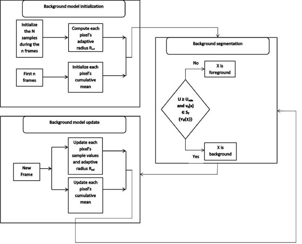
Fig.3. Functional architecture of the system. Here, all the parts of the system are shown.

The justification of the choice of value n has been mentioned in section IV.A. We also introduce the pixel counting mechanism which classifies as background a pixel that stays in foreground for more than countermax consecutive frames. This enables to boost up ghost elimination. To clearly illustrate how our approach eliminates ghost quicker than the original ViBE, we have used the winter Driveway dataset where two cars are at a stationary position for a long period (more than 1800 frames) before one of the two decides to move. The following observations have been made:

• The original ViBE proposed in 2011 (see line c of Figure 4) needs a longer period (more than 600 frames) to eliminates ghost apparition
• For version proposed in 2014 by the same author (see line d of Figure 4), ghost phenomenon elimination is much better. However the accuracy and quality of results have decreased.
• On the other hand, EFF-ViBE (see line e of Figure 4) needs less than 200 frames to perform the same task. In addition, the detected ghost is quickly eliminated (already eliminated at frame 2100) while it is still present at frame 2100 and at frame 2200 in both original and improved ViBE. The approach therefore outperforms the existing ViBE algorithms so can be adopted in complex background.

B. Effect of Adaptive Radius

As said earlier, for complex dynamic background, the radius should be increased appropriately, so that the background cannot be easily detected as foreground. This is because in basic ViBE algorithm, model matching always uses a fixed global radius. Yet, Le Chang et al[31] have shown by experiments that the simple radius policy ignores the complexity of the local environment and the uncertainty of changes. So it is therefore difficult to detect the target effectively in complex environment. That is why our third contribution consists of computing for each pixel a modified adaptive radius (we have decided to denote Rad) that depends on a variable parameter dmean computed using equation 9. It also uses fixed parameters εd = 0.08, εd = 0.35, δ = 5.

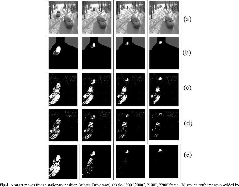
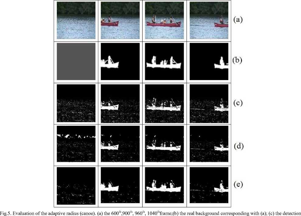
the dataset; (c) the detection results of the original ViBE; (d) the detection results of improved version of ViBE;(e) the detection results of EFF-ViBE proposed method.

To illustrate the effect of adaptive radius we have used the canoe data-set which consists of a canoe moving on sea disturbed by win that creates small waves on the sea surface. The following observations have been made:

• Normally the disturbance at the sea surface belongs to background but the original ViBE (see line c of Figure 5) tends to detect it as foreground
• The improvement (2014) tries to solve this failure (see line d of Figure 5), but the quality of the detected moving boat becomes poorer.
• EFF-ViBE on other hand solves these problems by computing the radius in an adaptive manner, consequently the effect of the waving background

is considerably reduced (see line e of Figure 5). Once more our approach outperformed original ViBE so can be used in complicated background.

C. Measure of Performances

We have recorded the precision, recall and F-measure of nine algorithms: the original ViBE algorithm, the execution of ViBE using cumulative mean and pixel counting mechanism, the execution of ViBE using adaptive radius, the proposed EFF-ViBE method and some challenging algorithms such as Codebook[17], KDE[14], MOG[6], PBAS[36] and SUBSENSE[37]. The results are shown in Table 2, Table 3 and Table 4.

results of the original ViBE;(d) the detection results of improved version of ViBE; (e) the detection results of EFF-Vibe proposed method.

The datasets used are those of CDNet 2014 and to have the results we have used the BMC-wizard software to compute those values. The process is as follows, we take the segmented images obtained by the chosen algorithm as first set of parameters and the second set of parameters to the BMC-wizard is the original ground truth of the input data provided by the dataset.

Mathematically, the precision Pr , recall R and the F-measure F - measure are computed using the formula

Pr ecision ( Pr ) = ——— ^v ’ TP + FP

Re call ( R ) =

TP + FN

F - MeasuredF ) =

2 x Pr x R Pr + R

where TP denote the number of foreground pixels truly classified as foreground, FP the number of background pixels wrongly classified as foreground and FN the number of foreground pixels wrongly classified as background.

• Quantitative analysis

The analysis of Table 2 shows how EFF-ViBE performs in terms of recall compared to the mentioned algorithms and it can be seen that it outperforms all the chosen algorithms with an average percentage of 65% of the cases (i.e among the 53 different challenging background situations proposed by the dataset) except PBAS algorithm where it outperforms only on 30% of the cases. The same observations can be made on Table 3, and here the results are even better for the average percentage of out-performance is about 90% for the other algorithm and 50% for PBAS algorithm. Finally combining these results to measure the F-measure (also called F-score) gives rises to Table 4 where the average percentage of outperformance is 85% for other algorithms and 40% for PBAS algorithm.

• Qualitative analysis

After having analyzed quantitatively the results, let us look at the quality aspect. Figure 6 presents the results obtained from different executions of algorithms for frames taken randomly in four datasets namely blizzard (1), park (2), sofa (3) and turnpike (4). Line (A) is the input frame, Line (B) is the ground truth image, Line (C) execution of PBAS algorithm, Line (D) execution of Subsense algorithm, Line (E) execution of Original ViBE algorithm, Line(F) execution of improved ViBE algorithm with n frames initialization, Line (G) execution of adaptive ViBE algorithm and Line (H) execution of EFF-ViBE algorithm.

It can therefore be seen how accurate are our proposed approach results compared to the other algorithms in relation to the ground truth image.

We can also notice that, even though at the quantitative analysis, the PBAS results were outperforming our approach; it is no more the case if we analyze the pictures. This was because PBAS detects a lot of background pixel as foreground pixel which was leading to modification of detection parameters (TP, FP and FN) and consequently good quantitative results were obtained.

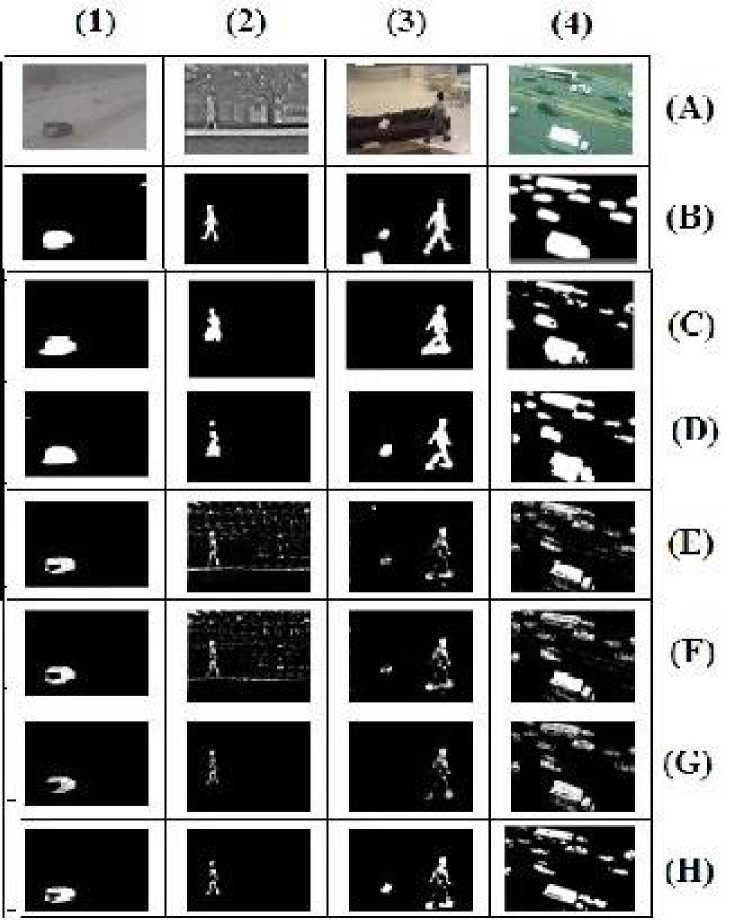
Fig.6. Analysis of results

Table 2. Recapitulating table of Recall

Category	Dataset	PBAS	SUBSENSE	ViBE	ViBE A.	ViBE I.	EFF-ViBE
Bad weather	blizzard	0.508	0.508	0.503	0.503	0.503	0.506
	skating	0.535	0.535	0.528	0.528	0.532	0.536
	snowfall	0.498	0.508	0.481	0.506	0.508	0.506
	wet snow	0.507	0.506	0.504	0.509	0.501	0.507
Baseline	highway	0.664	0.599	0.570	0.577	0.570	0.598
	office	0.613	0.582	0.548	0.591	0.599	0.553
	pedestrians	0.707	0.518	0.611	0.632	0.658	0.521
	pet2006	0.542	0.544	0.527	0.521	0.527	0.542
Camera jitter	badminton	0.607	0.529	0.529	0.521	0.514	0.549
	boulevard	0.565	0.519	0.516	0.557	0.549	0.513
	sidewalk	0.565	0.526	0.516	0.517	0.516	0.523
	traffic	0.577	0.545	0.571	0.550	0.545	0.579
Dynamic background	boats	0.513	0.513	0.502	0.508	0.505	0.509
	canoe	0.525	0.506	0.536	0.535	0.530	0.530
	fall	0.643	0.544	0.541	0.529	0.526	0.559
	fountain1	0.566	0.502	0.505	0.525	0.524	0.508
	fountain2	0.669	0.502	0.526	0.523	0.524	0.503
	overpass	0.554	0.512	0.511	0.511	0.511	0.512
Intermittent object motion	abandon B.	0.543	0.533	0.479	0.488	0.497	0.524
	parking	0.534	0.500	0.517	0.519	0.513	0.500
	sofa	0.710	0.576	0.609	0.604	0.590	0.770
	streetlight	0.615	0.520	0.552	0.549	0.542	0.570
	tram stop	0.553	0.526	0.512	0.507	0.515	0.574
	Win.D.W.S.	0.557	0.501	0.538	0.535	0.531	0.602
Low frame rate	port017fps	0.534	0.499	0.508	0.507	0.507	0.500
	tram C.	0.544	0.512	0.534	0.532	0.530	0.515
	Tunnel E.	0.514	0.500	0.515	0.514	0.514	0.515
	turnpike	0.589	0.533	0.547	0.544	0.541	0.538
Nigth video	bridge E.	0.542	0.501	0.501	0.503	0.502	0.503
	busy B.	0.534	0.501	0.501	0.501	0.501	0.501
	fluid high.	0.581	0.505	0.503	0.548	0.543	0.543
	StreetC.A.N.	0.510	0.503	0.502	0.502	0.502	0.502
	tramstation	0.551	0.514	0.508	0.518	0.508	0.508
	wint. Street	0.604	0.508	0.525	0.525	0.539	0.510
PTZ	Cont. p.	0.540	0.507	0.518	0.505	0.524	0.522
	Intermi. p.	0.527	0.511	0.515	0.512	0.519	0.521
	Cam. PTZ	0.548	0.541	0.532	0.522	0.517	0.531
	Zoom	0.586	0.505	0.438	0.439	0.450	0.458
Shadow	backdoor	0.599	0.542	0.541	0.538	0.536	0.525
	bungalows	0.651	0.589	0.583	0.581	0.577	0.561
	bustation	0.728	0.567	0.566	0.564	0.566	0.526
	copy M.	0.675	0.655	0.537	0.536	0.532	0.578
	cubicle	0.683	0.558	0.621	0.619	0.612	0.532
	people S.	0.740	0.606	0.588	0.583	0.581	0.576
Thermal	corridor	0.738	0.622	0.604	0.601	0.590	0.610
	dining r.	0.699	0.614	0.612	0.607	0.594	0.670
	lakeside	0.634	0.538	0.548	0.545	0.531	0.589
	library	0.612	0.591	0.567	0.564	0.555	0.624
	park	0.670	0.509	0.628	0.503	0.627	0.677
Turbulence	turbulence0	0.533	0.502	0.500	0.5003	0.500	0.501
	turbulence1	0.513	0.501	0.503	0.503	0.503	0.518
	turbulence2	0.500	0.501	0.501	0.501	0.501	0.500
	turbulence3	0.527	0.506	0.504	0.504	0.503	0.529

Table 3. Recapitulating table of precision

Category	Dataset	PBAS	SUBSENSE	ViBE	ViBE A.	ViBE I.	EFF-ViBE
Bad weather	blizzard	0.698	0.703	0.714	0.714	0.714	0.714
	skating	0.539	0.634	0.632	0.634	0.692	0.692
	snowfall	0.497	0.704	0.472	0.715	0.545	0.711
	wet snow	0.651	0.655	0.631	0.548	0.507	0.645
Baseline	highway	0.867	0.854	0.844	0.844	0.842	0.852
	office	0.833	0.839	0.834	0.594	0.616	0.827
	pedestrians	0.746	0.856	0.592	0.627	0.693	0.848
	pet2006	0.833	0.858	0.857	0.590	0.621	0.843
Camera jitter	badminton	0.612	0.632	0.616	0.590	0.637	0.639
	boulevard	0.677	0.694	0.623	0.690	0.686	0.567
	sidewalk	0.554	0.545	0.511	0.531	0.531	0.538
	traffic	0.687	0.688	0.678	0.687	0.684	0.679
Dynamic background	boats	0.702	0.699	0.544	0.575	0.553	0.628
	canoe	0.659	0.654	0.629	0.629	0.628	0.639
	fall	0.643	0.848	0.669	0.657	0.666	0.648
	fountain1	0.817	0.763	0.612	0.688	0.687	0.633
	fountain2	0.837	0.821	0.699	0.705	0.703	0.807
	overpass	0.826	0.801	0.728	0.740	0.737	0.792
Intermittent object motion	abandon B.	0.514	0.513	0.494	0.496	0.499	0.509
	parking	0.507	0.503	0.506	0.506	0.506	0.504
	sofa	0.652	0.873	0.884	0.878	0.885	0.824
	streetlight	0.534	0.608	0.521	0.521	0.524	0.522
	tram stop	0.509	0.508	0.502	0.501	0.503	0.506
	Win.D.W.S.	0.737	0.518	0.689	0.691	0.686	0.675
Low frame rate	port017fps	0.543	0.440	0.530	0.530	0.528	0.557
	tram C.	0.530	0.529	0.533	0.532	0.532	0.529
	Tunnel E.	0.545	0.504	0.573	0.573	0.573	0.573
	turnpike	0.569	0.601	0.598	0.598	0.598	0.598
Nigth video	bridge E.	0.521	0.504	0.508	0.517	0.513	0.521
	busy B.	0.523	0.506	0.511	0.513	0.512	0.511
	fluid high.	0.631	0.542	0.542	0.617	0.620	0.620
	StreetC.A.N.	0.631	0.627	0.590	0.579	0.579	0.596
	tramstation	0.585	0.575	0.569	0.553	0.579	0.569
	wint. Street	0.558	0.519	0.515	0.516	0.531	0.536
PTZ	Cont. p.	0.559	0.539	0.539	0.513	0.562	0.554
	Intermi. p.	0.532	0.552	0.535	0.537	0.551	0.558
	Cam. PTZ	0.529	0.583	0.550	0.565	0.581	0.574
	Zoom	0.596	0.516	0.423	0.424	0.425	0.430
Shadow	backdoor	0.845	0.829	0.775	0.779	0.776	0.822
	bungalows	0.777	0.790	0.746	0.749	0.758	0.785
	bustation	0.740	0.841	0.604	0.610	0.617	0.857
	copy M.	0.712	0.905	0.708	0.721	0.713	0.884
	cubicle	0.818	0.879	0.660	0.662	0.677	0.889
	people S.	0.878	0.877	0.674	0.672	0.680	0.880
Thermal	corridor	0.869	0.911	0.937	0.937	0.935	0.868
	dining r.	0.794	0.849	0.802	0.818	0.860	0.842
	lakeside	0.784	0.875	0.879	0.882	0.910	0.890
	library	0.634	0.816	0.818	0.816	0.820	0.816
	park	0.668	0.738	0.687	0.527	0.724	0.678
Turbulence	turbulence0	0.609	0.679	0.529	0.527	0.530	0.631
	turbulence1	0.541	0.659	0.561	0.561	0.558	0.675
	turbulence2	0.501	0.721	0.509	0.509	0.512	0.720
	turbulence3	0.645	0.651	0.598	0.599	0.598	0.642

Table 4. Recapitulating table of F-measure

Category	Dataset	PBAS	SUBSENSE	ViBE	ViBE A.	ViBE I.	EFF-ViBE
Bad weather	blizzard	0.588	0.590	0.590	0.590	0.590	0.592
	skating	0.537	0.604	0.575	0.577	0.601	0.604
	snowfall	0.498	0.590	0.476	0.591	0.526	0.591
	wet snow	0.570	0.572	0.560	0.528	0.504	0.567
Baseline	highway	0.752	0.704	0.686	0.685	0.680	0.703
	office	0.706	0.687	0.661	0.593	0.608	0.662
	pedestrians	0.743	0.645	0.601	0.629	0.675	0.645
	pet2006	0.657	0.666	0.653	0.554	0.570	0.666
Camera jitter	badminton	0.609	0.576	0.569	0.554	0.569	0.590
	boulevard	0.616	0.593	0.564	0.616	0.610	0.539
	sidewalk	0.559	0.535	0.514	0.524	0.524	0.531
	traffic	0.627	0.608	0.620	0.611	0.607	0.625
Dynamic background	boats	0.593	0.591	0.522	0.539	0.528	0.562
	canoe	0.585	0.570	0.579	0.578	0.575	0.579
	fall	0.643	0.663	0.598	0.586	0.587	0.600
	fountain1	0.669	0.605	0.553	0.596	0.594	0.564
	fountain2	0.744	0.623	0.601	0.600	0.600	0.620
	overpass	0.663	0.625	0.600	0.605	0.603	0.622
Intermittent object motion	abandon B.	0.528	0.523	0.486	0.492	0.498	0.517
	parking	0.520	0.502	0.511	0.513	0.509	0.502
	sofa	0.680	0.694	0.721	0.715	0.708	0.795
	streetlight	0.572	0.524	0.536	0.534	0.533	0.545
	tram stop	0.530	0.517	0.507	0.504	0.509	0.538
	Win.D.W.S.	0.635	0.509	0.605	0.603	0.599	0.637
Low frame rate	port017fps	0.538	0.468	0.519	0.518	0.517	0.527
	tram C.	0.537	0.520	0.533	0.532	0.531	0.522
	Tunnel E.	0.529	0.502	0.543	0.542	0.542	0.543
	turnpike	0.579	0.565	0.571	0.570	0.568	0.571
Nigth video	bridge E.	0.531	0.502	0.504	0.510	0.507	0.512
	busy B.	0.529	0.503	0.522	0.507	0.507	0.506
	fluid high.	0.605	0.523	0.522	0.581	0.581	0.579
	StreetC.A.N.	0.564	0.558	0.542	0.538	0.538	0.546
	tramstation	0.567	0.543	0.537	0.535	0.539	0.537
	wint. Street	0.581	0.513	0.520	0.521	0.535	0.523
PTZ	Cont. p.	0.550	0.522	0.529	0.509	0.542	0.538
	Intermi. p.	0.530	0.531	0.525	0.524	0.534	0.539
	Cam. PTZ	0.538	0.561	0.541	0.542	0.547	0.551
	Zoom	0.591	0.511	0.430	0.431	0.432	0.443
Shadow	backdoor	0.701	0.656	0.637	0.636	0.634	0.641
	bungalows	0.708	0.674	0.655	0.655	0.655	0.655
	bustation	0.737	0.678	0.584	0.586	0.591	0.652
	copy M.	0.693	0.760	0.611	0.615	0.610	0.699
	cubicle	0.744	0.683	0.640	0.619	0.643	0.666
	people S.	0.803	0.717	0.628	0.625	0.622	0.696
Thermal	corridor	0.798	0.739	0.735	0.733	0.724	0.717
	dining r.	0.744	0.712	0.699	0.697	0.703	0.746
	lakeside	0.701	0.666	0.675	0.674	0.671	0.709
	library	0.622	0.685	0.670	0.667	0.662	0.708
	park	0.669	0.602	0.656	0.513	0.672	0.677
turbulence	turbulence0	0.568	0.577	0.514	0.513	0.514	0.558
	turbulence1	0.527	0.569	0.530	0.531	0.529	0.585
	turbulence2	0.500	0.591	0.505	0.505	0.506	0.590
	turbulence3	0.580	0.570	0.547	0.547	0.547	0.580

VI. Conclusion

This paper has presented an efficient background subtraction algorithm based of ViBE for complex background. For that, we studied related work done on the original ViBE algorithm with some improvements. Later on, the EFF-ViBE proposed method has been explained in details with all the needed parameters. It combines an improved ViBE that uses a cumulative mean and a pixel counting mechanism to quickly eliminate ghost and on an adaptive ViBE that computes an adaptive radius depending on background variation. Finally, the obtained results have been presented showing the efficiency of the method in comparison with the existing ones. With an average frame rate of 30 fps it can also been used in real time applications. For future work, we intend to speed-up the proposed method and see how it can be adapted for further applications.

Список литературы EFF-ViBE: an efficient and improved background subtraction approach based on ViBE

S. S. Hossain, S. Khalid, C. Nabendu, Moving Object Detection Using Background Subtraction, Springer Briefs in Computer Sciences Sciences, Sprnger, Cham, 2014.
G. Yao, T. Lei, J. Zhong, P. Jiang, W. Jia, Comparative evaluation of background subtraction algorithms in remote scene videos capturedby mwir sensors, Sensors (2017).
F. Zeng, G. Zhang, J. Jiang, Text image with complex background ﬁltering method based on harris corner-point detection, journal of software 8 (8) (2013).
D. Li, Y. Li, F. He, S. Wang, Object detection in image with complex background, Third International Conference on Multimedia Technology(2013).
O. Barnich, M. V. Droogenbroeck, Vibe: A powerful random technique to estimate the background in video sequences, International Conference on Acoustics, Speech, and Signal Processing (ICASSP)(2009) 19–24.
C. Stauffer, E. Grimson, Adaptive background mixture models for real-time tracking, Computer Vision and Pattern Recognition (1999) 246–252.
B. Han, X. Lin, Update the GMMs via adaptive Kalman filtering,International Society for Optical Engineering (2005) 1506–1515
Y. Hong, Y. Tan, J. Tian, J. Liu, Accurate dynamic scene model for moving object detection, International Conference on Image Processing (ICIP) (2007) 157–160.
W. Zhang, X. Fang, X. Yang, J. Wu, Spatio-temporal Gaussian mixture model to detect moving objects in dynamic scenes., Journal of Electronic Imaging (2007).
P. Tang, L. Gao, Z. Liu, Salient moving object detection using stochastic approach filtering, Fourth International Conference on Image and Graphics (ICIG (2007) 530–535.
M. Harville, A framework for high-level feedback to adaptive, perpixel, mixture-of-Gaussian background models, 7th European Conference on Computer Vision (ECCV) (2002) 543–560
M. Cristani, V. Murino, A spatial sampling mechanism for effective background subtraction, 2nd International Conference on Computer Vision Theory and Applications (VISAPP) (2007) 403–410
A. Elgammal, D. Harwood, L. Davis, Non-parametric model for background subtraction, European Conference on Computer Vision(2000).
A. Elgammal, R. Duraiswami, D. Harwood, L. Davis, Background and foreground modeling using nonparametric kernel density estimation for visual surveillance, Proceedings of the IEEE 90 (2002) 1151–1163.
Park, C. Lee, Bayesian rule-based complex background modeling and foreground detection optical engineering, Optical Engineering (2010)
P. Angelov, P. S. Tehran, R. Ramezani, An approach to automatic real-time novelty detection, object identification, and tracking in video streams based on recursive density estimation and evolving Takagi-Sugeno Fuzzy systems, International Journal of Intelligent Systems (2011) 189–205.
K. Kim, T. H. Chalidabhongse, D. Harwood, L. Davis, Real-timeforeground background segmentation using codebook model, Real time imaging 11 (2005) 172–185.
N. M. Oliver, B. Rosario, A. P. Pentland, A bayesian computer vision system for modeling human interactions, IEEE transactions on pattern analysis and machine intelligence 22 (2000) 831–843.
D. Kuzin, O. Isupova, L. Mihaylova, Compressive sensing approaches for autonomous object detection in video sequences, Sensor Data Fusion: Trends, Solutions, Applications (SDF) (2015).
V. Cevhe Aswin, S. M. F., D. Dikpal, R. R. G., B. R. Chellappa,Compressive sensing for background subtraction, European Conferenceon Computer Vision (2008) 155–168.
V. Cevher, A. Sankaranarayanan, M. F., D. Dikpal, R. R. G., B. R. Chellappa, Background subtraction using spatio-temporal group sparsity recovery, European Conference on Computer Vision(2008) 155–168.
A. Azeroual, K. Afdel, Ieee transactions on circuits and systems for video technology: Background subtraction based on low-rank and structured sparse decomposition, IEEE Trans. Image Process 24 (08) (2017) 2502–2514.
A. Azeroual, K. Afdel, Fast image edge detection based on faber schauder wavelet and otsu threshold, Heliyon 3 (2017), doi: 10.1016/j.heliyon.2017.e00485.
M. Nishio, C. Nagashima, S. Hirabayashi, A. Ohnishi, K. Sasaki, T. Sagawa, M. Hamada, T. Yamashita., Convolutional auto-encoderfor image denoising of ultralow-dose ct, Heliyon 3 (2017), doi:10.1016/j.heliyon.2017.e00393.
M. Braham, M. V. Droogenbroeck, Deep background subtraction with scene-speciﬁc convolutional neural networks, International Conference on Systems, Signals and Image Processing (2016).
Y. LeCun, L. Bottou, Y. Bengio, P. Haﬀner, Gradient-based learning applied to document recognition, Proceeding of IEEE 86 (1998) 2278–2324.
O. BARNICH, M. V. DROOGENBROECK, Vibe : A universal background subtraction algorithm for video sequences., IEEE Transactions on Image Processing (2011) 1709–1724.
A. Elgammal, D. Harwood, L. Davis, Non-parametric model for background subtraction, 6thEuropean Conference on Computer Vision Part II, Springer 1843 (2000) 751–767.
H. Wang, D. Suter, A consensus-based method for tracking: Modeling background scenario and foreground appearance, Pattern Recognition40 (2007) 1091–1105.
H. Batao, Y. Shaohua, An improved background subtraction method based on vibe, Chinese Conference on Pattern Recognition, Springer 662 (2016) 356–368
L. Chang, Zhenghua, Y. Ren, Improved adaptive vibe and the application for segmentation of complex background, Hindawi Publishing Corporation, Mathematical Problems in Engineering (2016).
Itseez, Open source computer vision library, https://github.com/itseez/opencv (2015).
Y. Wang, G. P. M. Jodoin, F. Porikli, J. Konrad, P. Ishwar, Y. Benezeth, P. Ishwar, Cdnet 2014: An expanded change detection benchmark dataset, 2014 IEEE Conference eon computer Vision and Pattern Recognition Workshops (2014) 16–21.
B. Laugraud, vibe-sources, source code in c/c++! original implementation. example for opencv, University of Liege, Belgium, http://orbi.ulg.ac.be /bitstream/2268/145853/5/vibe- sources.zip (2014).
A. Sobral, Bgslibrary: An opencv c++ background subtraction library,In Proceedings of the 2013 IX Workshop de Viso Computacional, Rio de Janeiro, Brazil (2013) 3–5.
M. Hofmann, P. Tiefenbacher, G. Rigoll, Background segmentation with feedback: The pixel-based adaptive segmenter, In Proceedings IEEE Computer Society Conference on Computer Vision and Pattern Recognition Workshops, Providence , RI, USA (2012).
St-Charles, G. A. Bilodeau, R. Bergevin, Flexible background subtraction with self-balanced local sensitivity, In Proceedings of the 27th IEEE Conference on Computer Vision and Pattern Recognition, Columbus, OH, USA (2014) 414–419.

Еще

Статья научная