Effect of Maintenance on Computer Network Reliability

Published Online August 2014 in MECS DOI: 10.5815/ijcnis.2014.09.02

Currently, computer networks are inescapable in any large organization, where they are organized so as to form powerful internal means of communication. At the time of the new information technologies, dependability plays an important role in these communication networks where the expected service must be continuous and without interruption. In this context, the reliability parameter proves to be fundamental to evaluate the performances of such systems.

Dependability [1, 2] can be defined as the ability of an entity (or system) to deliver service that can be justifiably trusted. So, this concept is crucial to ensure continuity of correct service, particularly through the reliability estimation obtained by reliability laws.

Reliability [3] can be defined as the ability of an entity (equipment, component, subsystem and system) to remain functional. It specifies that no failures will occur during a stated time interval. Reliability is a quantitative greatness and requires the knowledge of distribution of lifetime, given by laws of reliability.

In order to lengthen the life of the system and improve its reliability, we must master the risk of failure, thus; the maintenance process appears as essential to manage these risks and ensure the good functioning of the system.

Several studies have been made to improve system reliability evaluated by the Exponential and Weibull distribution [4-6]. As the system reliability depends on efficiency of maintenance, so it is necessary to choose an effective maintenance strategy that will reduce failures and improve reliability of the system. For it, several literatures propose the models to assess the effects of maintenance on system reliability [7, 8].

In this paper, we examine the reliability evaluation of a computer network through the reliability models; thereafter, we determine a proper maintenance policy in order to increase system reliability.

The following section describes the computer network concerned by this study. We present, in particular, the data obtained after watching the network. The third section presents the three reliability models, given in the form of the laws Exponential, of Weibull and Normal. These laws were adopted because they intervene most frequently in data analysis of life and in the estimation of reliability. The result is the evaluation of the reliability corresponding to each law of the network studied and a comparison of three models is made by calculating the determination coefficient which to judge the most appropriate model of network reliability .

The following of our study, aims to improve the reliability of the system studied by defining a good maintenance strategy through a model of the most common competing risks in maintenance [9, 10] called the Alert Delay model. At the end, measures of dependability such as MTBF (Mean Time Between Failures) and reliability are calcu lated to assess the effectiveness of strategies for maintenance and then validate the model studied.

• II.    Reliability Laws

In this section we will state at first the main laws of reliability, and then we will present the adopted laws.

• A.    State of the Art

Among the various usual laws reliability, we have identified the following laws: the Log-normal law (Galton law or Gibrat law), the Gamma law, the Gompertz-Makeham law, the Birnbaum-Saunders law, the Chi-squared law, the Beta law, the Exponential law, the Weibull law and the Normal law.

Lognormal law: a continuous random variable and positive T is distributed according to a lognormal distribution if its natural logarithm is distributed according to a normal distribution [3]. This distribution is widely used to model data of life; especially in mechanical fatigue failures .The lognormal distribution is a law with two parameters.

Gamma law: it is a law that can model a system of three phases of life, but it is inadequate for modeling human life (decrease too fast).It is applied as a probability model for predicting the lifetime of the devices which are subject to wear such as motor vehicles or mechanical devices. The gamma distribution is a law with two parameters, which can be generalized by several laws such as the exponential [11].

Gompertz-Makeham law: in terms of reliability theory the Gompertz-Makeham law of mortality represents a failure law where the hazard rate is a mixture of failure distribution of non-aging and the failure distribution of aging with exponential increase in failure rates [12].

As the Weibull distribution, the Gompertz law represents a process of change of state of which the risk varies monotonically as a function of time.

Birnbaum-Saunders law: to characterize failure due to crack propagation by fatigue, Birnbaum and Saunders (1969) proposed a distribution of life based on two parameters [13]. This distribution can be used to model lifetime data and it is widely applicable to model failure times of fatiguing materials [14, 15].

Chi-squared law: Chi-squared law, or the Pearson, does not serve to model directly the reliability, but essentially in the calculation of confidence limits around a measured failure rate. It is well-known for testing the goodness-of-fit. Chi-squared law is characterized by a positive parameter called degree of freedom and defined that for positive values [16].

Beta law : this law is, inparticular, the probability that material survives until time t , when you try n material, hence its interest in assessing the duration of reliability testing. The Beta law has two parameters and this law presents the advantage to benefit from parameters of shape: these latter allow giving to the beta law a shape close to other laws [17].

Exponential law: this model has many applications in various fields. It perfectly describes the life of materials that undergo brutal and chance failures [11], and is commonly used in electronics reliability to describe the period during which the failure rate of the equipment is considered as constant [18].

Weibull law : the Weibull distribution is often used in the field of the analysis of life, thanks to its flexibility, it allows to represent at least approximately infinite probability distributions [19].This distribution is named after the Swedish professor Walodi Weibull, which showed the usefulness of this distribution to model various types of data [3, 11].

Normal law: in reliability, the normal distribution is used to represent the lifetime distribution of devices at the end of life (wear) [20, 21]. This is one of the main probability distributions [22], and is a theoretical distribution, in that it is a mathematical idealization.

• B.    Adopted Reliability Laws

In analysis reliability and among distribution functions, our choice carried on the three most widespread reliability models, given in the form of the Exponential laws, of Weibull and Normal.

In general, these popular models are dedicated to specific applications (electronic, mechanical, etc...) and we propose to apply them to the real computer network.

Definition of the exponential model: the exponential distribution is defined by a single parameter, the failure rate λ, where λ is a strictly positive real constant [18].

Let «exp» classical exponential function. The reliability function R(t) also called survival function where t is the time unit ( t ≥ 0) is expressed by [20]:

R (t) = exp (- λ t) (1)

Definition of the Weibull model: the basic Weibull model [3] has two parameters, the shape parameter (β) and the scale parameter (η):

• -    в : shape parameter в > 0; it defines the type of degradation phenomenon in question.

• -    n : scale parameter n > 0, and is a unit of time.

Extensions are introduced by adding parameters [23]. Among them, the location parameter (γ, γ>=0) is considered giving the more general form of the Weibull model: the three parameters (γ, β, η) of the Weibull distribution [3].

The general Weibull model is a reliability law with the three parameters that permit to describe the three phases of system life (youth or infant mortality, useful life, wear-out), widely known as the bathtub curve in the dependability domain [18, 19, 24].

The description of the three phases of a device life is specified through the shape parameter β, as follows [11, 19]:

• -    If the failure rate decreases over time then в <1, and the component is in its infantile period or youth defects.

• -    If the failure rate is constant over time then в =1, and is called the period of useful life or random of failures. Components follow an exponential distribution.

• -    If the failure rate increases with time then в >1, and the

period is said to wear out or aging.

Note there are a variety of symbols in literature for the same parameters. For example, α is designing for the shape parameter and β for the scale parameter [23].

There are many variants and we adopt the three parameters Weibull distribution. In this case, the formula for the survival function is [22]:

R(t)= exp - ((t – γ )/ η ) ^β.                  (2)

Definition of the Normal model: this distribution was highlighted by Gauss and allows modeling many biometric studies. Its probability density draws a curve called the bell curve or Gaussian curve. It is defined by two parameters, the mean ( µ ) and the parameter σ, where σ is either positive or null:

• -    ц : determine the position of the curve.

• -    c : determine the scale ,the values dispersion around the mean.

The reliability function is given by:

R(t)= 1 - φ ((t - µ )/ σ ) .                  (3)

Where μ is the mean value; σ is the standard deviation and φ is the distribution function of the normal distribution [20].

• III.    Specification of the Computer Network

The considered computer network, localized in an industrial company, consists of PCs and server interconnected. In the context of dependability, a preliminary analysis of dysfunctions of the network is necessary.

• A.    Principle of the Dysfunctions Analysis

Having a real computer network and using a utility called "The Dude" [25], we could collect data on different network failures and their duration for a fixed period. The Dude is a network monitoring program; it automatically analyzes all devices (printers, switches, PCs, serv-ers,…etc) within an intranet network to draw a map of the network (Fig. 1).

Fig 1: The network map.

The Dude program also monitors all services and alerts in case of failures on any device.

Thus, we have identified the various failures as well as their durations for seven days observation [26]. For ex- ample, consider a part of the network with two failures (Fig. 2); the failure 5 (in red color) ‘Service disk on MBAREK (a computer name in the network) is now not available’ begins at 11:22:35 and finish at 11:26:06, for a duration of 211 seconds.

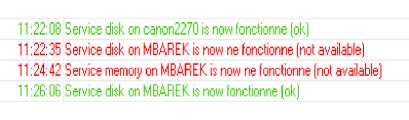
Fig 2: The failure 5 in the third day.

• B.    Identification of Failures

After observation of the network, we had 351 failures from 9 hours until 15 hours for seven days. At each detected failure is associated its duration, calculated (in seconds) from the beginning and end of the failure, during the observation period.

The following table (Table 1) shows all failures detected in the 6th day.

Table 1: Example of identified failures with duration
Failures	Start of failure	End of failure	Duration
3th day
Failure 5	11:22:35	11:26:06	211
6th day
Failure 1	08:59:03	08:59:23	20
Failure 2	09:22:29	09:25:59	210
Failure 3	09:31:55	09:32:46	51
Failure 4	09:32:10	09:33:30	80
Failure 5	10:26:38	10:30:09	211
Failure 6	11:37:29	12:05:23	1674
Failure 7	11:37:29	12:05:23	1674
Failure 8	11:58:55	12:02:22	207

All durations of failures on each day and the duration of all failures reported during the observation period are given in the following Table:

Table 2: Failures with duration

Day	Duration of failures
1st day	267697
2nd day	153163
3rd day	562827
4th day	167013
5th day	39110
6th day	4127
7th day	3541
Failure duration	1197478

These data allowed us to generate the parameters of the selected models and calculate the network reliability.

• IV.    Reliability Models for the Network

  We applied the three adopted reliability models to the computer network.

  To estimate the network reliability, and to test the choice of model, we have developed a software [26], including a database of failures; this software allows the generation of parameters (Fig. 3), estimating the network reliability with its associated function (Fig. 4), according to the three models and during an interval time [0, 1008] (6hrs of failures/ day, for 7 days).

  A. Generation of Parameters for Reliability Models

  Application of the exponential model: from the observation of times and failures, we calculate the MTBF which represents the mean time between failures, formula for calculating the MTBF is [18, 27, 28]:

  
  

  for the time t = 3628800 sec or t = 1008 hrs .

  
  

  MTBF =

  
  

  Total up time ( TBF ) Number of failures

  
  
  
  

  Exponential          Weibull            Normal

  

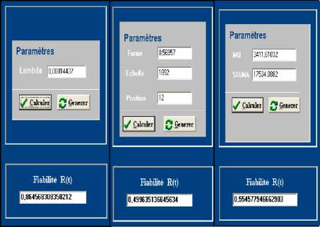
  Fig 3: Parameters and reliability of each model.

  
  

Knowing that TBF is calculated by:

TBF = duration of observation – duration of failures. (5)

In this case, the parameter λ of the exponential model is the inverse of the value of the MTBF.

We obtain:

• -    TBF = 2431322.

• -    MTBF = 6926.8433.

• -    A = 0.00014437.

Application of the Weibull model: given the complexity of calculating the three parameters of the Weibull law, we used a classical tool ‘Easyfit’ [29], well known for the calculation of distribution functions.

So from the data of failures, we obtain:

• -    The shape parameter, the value 0.56957 (в being less than 1, we are in the period of youth).

• -    The scale parameter, the value 1892.

• -    The location parameter, the value 12.

By taking into account the β value, we can say that in the material part some components are in its infant period, also in the software part where at the beginning there are undetected bugs that make the failure decrease progressively of their detection and correction.

Application of the Normal model: considering the values (xi) the duration of failures, values ni) representing the corresponding effective for a duration of failure concerned and (n) the number of failures, the values of two parameters ц and о are generated: the mean ц is calculated out conventionally by (xi.ni) / n and σ represents the standard deviation.

We obtain:

• -    ц = 3411.61823.

• -    о = 17534.0882.

• B.    Network Reliability

  As the reliability is a function of time, we considered the time t = 1008 hours with unit of time equal to 100.

Following parameters (Fig. 3) of each law and by application of the respective formulas (1), (2), (3), the developed software calculates the reliability of each model

The following figure gives the curves (Fig. 4) for each reliability models and for the time duration.

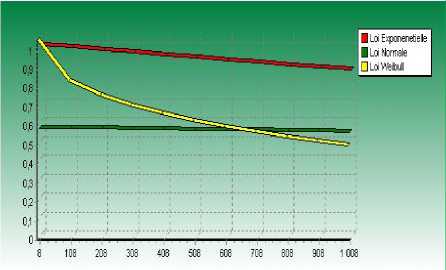
Fig 4: Representation of reliability models.

Note that for t = 0, reliability is equal to 1, the commissioning of the system does not encounter any failure in the exponential and Weibull laws. Then reliability decreases as the lifetime of the system decreases over time.

The reliability presented by the Weibull law is declining relative to other laws, failures occur quickly due to youth defects because β <1.

• C.    Comparison of Models and Interpretation

To test the choice of model, we apply the notion of determination coefficient (r2) [30], well known in the domains of descriptive statistical. The coefficient of determination allows judging the model through its value: when the determination coefficient (r²) is equal or close to 1, then the model is accepted. The coefficient of determination (r²) is expressed by the general formula [30]:

r ²

[nZ ',MZ -„x. )(z Ly)]'

nz >2-(zLy)'

n z m x - (z ^) '

In our context of reliability, we consider

- X i as the time unit,

• -    y i as the reliability function for x , ,

• -    n as the number of calculation units.

As the interval time is from 0 to 1008, the step is 100 and we deduce n =12 by adding the last value. The software gives the value of the function y i for each x i (see the obtained values in the fig. 4).

From these values and with the formula (6), the developed software can calculate the determination coefficient of each law presented in fig. 5:

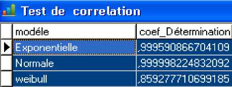
Fig 5: Determination coefficient of three reliability model.

Following these results, we note that the coefficient of determination of both normal and exponential laws is closer to 1, with very little discrimination. This means that these two laws are best suited for the studied network reliability. The Weibull distribution is the least suitable model, which is coherent because this model is classically used in mechanical applications, where there are notions of wear.

Let us note, however; that the reliability attached to this model is close to the reliability associated with the normal distribution, as these values are calculated from parameters generated (from the data), while in the exponential law intervenes only in the failure rate calculated directly from the data. Indeed, the normal distribution is used to represent the distribution of lifetimes at the end of life (wear) because the failure rate is still increasing.

This explains that eventually the exponential law remains a powerful and interesting model.

• V.    Definition of Maintenance Policy

In order to lengthen the life of the system and improve its reliability, we must master the risk of failure, thus, the maintenance process appears as essential to manage these risks and ensure the good functioning of the system.

Thereby, the following of our study aims to improve the reliability of the system studied by defining a good maintenance strategy through a model of the most common competing risks in maintenance called the Alert Delay model.

• A.    Alert Delay Model

Definition of the Alert Delay model: this model allows situating the preventive maintenance policy compared to the occurrence of failure and after the alert; the choice of this model is that it allows also have an initial insight into the effectiveness of maintenance. The use of this model, can determine the time and the nature of the maintenance to be performed.

The system sends an alert just before failure, it requires delay ε to perform preventive maintenance after alert [31], is defined by:

Y= p Z+ ε                 (7)

Where

• -    Y is the duration of preventive maintenance (PM).

• -    Z is the duration of corrective maintenance (CM).

• -    p ⁶ [0,1], alert delivered in p Z.

Z and ε are two independent positive random variables.

This model is interesting because it considers that to have an effective preventive maintenance it should take place before the failure, what occurs when Y = p Z.

Similarly, for having a policy of ideal preventive maintenance, it must be performed as late as possible that is to say just before the failure, this can be expressed by a p close to 1.

Thus, the preventive maintenance will be efficient if the alert is not delivered too early and if the delay is short (p should be close to 1).

The alert delay model includes several particular cases:

• - If p = 0, Y = e, so Y and Z are independent.

• - If p = 1, Y = Z + e >Z, so only CM (failures) are ob

served.

• -    If there is not delay after the alert e =0, Y =p Z, so only PM are observed.

Our objective is to define a maintenance policy of the system studied to improve the reliability of the system. To do this, we will apply the model alert delay on the duration of failures given in table 2.

Application of the model Alert Delay: our approach is to vary the parameters of the model alert delay; this allows us to estimate, on the one hand, the duration of preventive maintenance or to observe a failure and, on the other hand, to determine the impact of time and the alert conducive to perform accurate and efficient maintenance [32].

These parameters are the alert delivered by the system p and the delay ε needed to perform the PM after the alert.

We consider the following random variations of the parameters (p, ε), knowing that p [0, 1].

• B.    Identification of the Maintenance Duration

We consider two interested cases following the random variations of the parameters ( p , ε ):

• - Case 1: p = 0.65 and e = 1000 .

• - Case 2: p =0.85 and e = 5000.

Using the assumption (7) alert delay Model and the data presented in table 2, we were able to estimate all possible duration of preventive maintenance for each value of ε and p. The results are shown in the following table:

Table 3: Duration of preventive maintenance

Duration of preventive maintenance
p = 0.65 and ε = 1000	p = 0.85 and ε = 5000
175003.05	232542.45
102027.55	137112.95
365365.45	481478.55
109558.45	146961.05
26421.5	38243.5
3682.55	8507.95
3301.65	8009.85
Number of maintenance
7 MP - 0 MC	5 MP - 2MC

Preventive maintenance is effective if it is performed as late as possible that is to say that the alert is not delivered too early and if the delay is short.

We notice in this table, that the durations of preventive maintenance are performed just before failure because the alert is not given too early and the delay is close to 1, therefore according to the alert delay model the maintenance is effective.

Occasionally failure may occur before preventive maintenance, this happens when Y >  Z and when the alert ( p ) is close to 1, in this case the probability of a corrective maintenance is greater than the probability to perform preventive maintenance.

For example in the case 2 where ( p = 0.85 and ε = 5000) some failures have occurred before preventive maintenance, in these conditions, we perform corrective maintenance. However, in case 1 where ( p = 0.65 and ε = 1000) we only perform preventive maintenance as ( Y <  Z )

• C.    Effects of Maintenance

Maintenance of the system is considered perfect where after maintenance, the system is refurbished, and we assume that the duration of maintenance is the availability of the system.

To evaluate the effectiveness of maintenance strategies the dependability measure the MTBF is estimated before and after performing maintenance [32].

Before maintenance, the MTBF has been calculated in the context of the exponential law and the MTBF of the system before maintenance was 6926.8433.

During duration of observation for t = 3628800 sec, the

MTBF of the maintenance strategy is calculated by the formula (4):

• -    For case 1: the MTBF 1 where p = 0.65 and e = 1000

is 406205.614.

• -    For case 2: the MTBF 2 where p = 0.85 and e = 5000 is 367991.9571.

  Before maintenance

  
  

  After maintenance

  
  

  MTBF 1

  
  

  MTBF 2

  
  

MTBF initial ------►

I_________________________________________________________

0         6926.84      367991.95    406205.61     3628800

Fig 6: The evolution of MTBF

After maintenance, it is clear that the value of MTBF is improved. However, a good maintenance strategy is that which makes it possible to increase the state of good functioning of the system and in our case; it is the MTBF 1 which is equal to 406205.614.

This explains why the level of system operation is improving rapidly in the first case, and the fact that performs preventive maintenance permits to rejuvenate the system thus to lengthen its lifetime.

To validate this maintenance strategy, we estimate the reliability of the system through the formula (1) for t = 1008 h, so we get the following results:

• -    For case1: Z 1 = 0.0000024618 and R 1 (t) = 0.99752157.

• -    For case 2: Z₂ = 0.0000027175 and R 2 (t) = 0.99726456.

According to these results (Fig. 7), the maintenance strategy has to significantly improve reliability of the system from 86% to 99% (for the two cases).

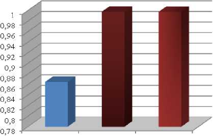
Before MP After MP After MP

(Casel) (Case 2)

Fig 7: Reliability of the system

For good maintenance strategy, we opt for the second strategy. Indeed, performing only the preventive maintenance will be very expensive.

In fact, preventive maintenance is intended to reduce the likelihood of failure but there is still a part of corrective maintenance.

It is, therefore, necessary to consider strategies that combine both: corrective maintenance and preventive maintenance.

• VI.    Conclusions

We presented in this paper, the estimation of the computer network reliability located in a local company, according three reliability models commonly used in other domains. In order to implement the adopted models, we used the parameters of these models, the actual historical data concerning of the data collected after observation of the network.

In basing on the determination coefficient, the final result has permit to make a comparison between the three models and decide on the most appropriate reliability model to the studied network.

The study showed that the exponential model is best suited to evaluate the reliability of computer networks.

Finally, we propose to establish a policy of effective and proper maintenance using a competing risks model the more used in the context of maintenance called the Alert Delay model. In this model; the decisions of maintenance are taken according the state of system degradation.

Indeed, the maintenance operations are realized when the level of the system degradation is detected by an alarm or a failure appears.

The objective of this study is to improve system reliability and consequently ensure its state of good functioning based on a good maintenance strategy.

To evaluate the effectiveness of maintenance strategies and validate the Alert Delay model, measures of dependability are calculated order to select duration of maintenance which can gives an optimal operation of the system and to lengthen the lifetime.

To achieve this objective, the notion of competing risks and the resulting models should be studied, among these models we test the Alert Delay exponentially model given that this law is the most appropriate for the study of computer networks, we will thus apply it in the field of maintenance.

• [1]    A. Avižienis, J.C. Laprie and B. Randell, “Fundamental Concepts of Dependability” In Proc. of the 3rd IEEE Information Survivability Workshop (ISW-2000), USA, pp. 7-12, October 24-26, 2000.

• [2]    G. Zwingelstein, “Sûreté de fonctionnement des systèmes industriels complexes,” Techniques de l’Ingénieur, S825v2 / S8251, 2009.

• [3]    A. Birolini, “Reliability Engineering: Theory and Practice”, Springer-Verlag, Sixth Edition, Berlin, 2010.

• [4]    K. Kołowrocki, Reliability of Large Multi-State Exponential Systems , Reliaility of Large and Complex Systems (Second Edition), pp. 221–248, 2014, ISBN: 978-0-08099949-4.

• [5]    K. Das, A comparative study of exponential distribution vs Weibull distribution in machine reliability analysis in a

  CMS design, Original Research Computers & Industrial Engineering, Vol.54, Issue 1, pp. 12-33, February 2008.

Rima Oudjedi Damerdji obtained her master degree in computer systems and network from University of Science and Technology of Oran, Algeria, in the year 2011.

Currently, she is pursuing her PhD studies in computer systems and network in the department of computer science, University of Sciences and Technology of Oran, Algeria.

Her major interest is in the dependability and maintenance of computer networks.

Myriam Noureddine is currently Assistant Professor in the department of computer science in the University of Sciences and Technology of Oran (USTO). Among her research interests, the dependability domain is important dealing with the failure diagnosis, the risk management and the system reliability, with application in industrial systems and computer networks.