Element-Based Computational Model

Published Online February 2012 in MECS DOI: 10.5815/ijmecs.2012.01.01

The following two quotes are the motivation for the research.

“For more than 30 years, researchers and designers have predicted the end of uniprocessors and their dominance by multiprocessors. During this time period the rise of microprocessors and their performance growth has largely limited the role of multiprocessors to limited market segments. In 2006, we are clearly at an inflection point where multiprocessors and thread-level parallelism will play a greater role...” [1]

“Since real world applications are naturally parallel and hardware is naturally parallel, what we need is a programming model, system software, and a supporting architecture that are naturally parallel. Researchers have the rare opportunity to re-invent these cornerstones of computing, provided they simplify the efficient programming of highly parallel systems.” [2]

Given the need for parallelism, is it not worth looking at previous attempts at parallel models? In the 1970s, the data-flow model was explored with some limited success [3]. This paper explores how to build on some of the concepts of the data-flow model. This new data-driven model has significant differences from the previous data-flow models, as described below, as well as being inherently parallel, which simplifies parallel programming.

Table 1: Comparison between Data-flow and Element

program graph edge node values	Data‐flow        Element‐based
	cyclic graph	acyclic graph
	finite	infinite
	pointer	element
	instruction	relation
	memory	elements
computation current state result of op selection	firing instruction	processing element
	values in nodes	active elements
	a value	a new element
	instructions	partial functions

As Hennessy [4] has pointed out, implementing a new architecture requires considerable resources. These are unavailable to us. The objective of this paper is to provide some evidence that it is worthwhile taking this research further, in the hope that others may see some potential in collaborating in this research. The method chosen to provide this evidence is to experiment with an example program and assess how the new model is likely to compare with the predominant instruction-based model.

The model is built on theory relating to functions and sets that forms both the basis of the model and a language to express programs. Developing the language is a research project on its own and its justification depends on acceptance of the model. For this reason the focus has been on the model. Understanding programs written in the language only requires an understanding of simple algebraic mathematical expressions. That is sufficient for this paper.

The paper reports experimental results of simulating some of the behavior of this model. These results suggest that such an architecture's performance scales well with increases in processors. An MPI [5] emulation is used to compute a matrix multiplication with increasing sizes and increasing numbers of processors. Based on given assumptions, an argument is made that an architecture based on this model scales linearly for the example.

The rest of the paper is broken up into three sections. The first given a brief description of the model and compares it with other architectures. The next section describes the research method. The final section evaluates the research and considers how to take the research further.

• II.    Model of Computation

• A.    Basics

In many ways our model is similar to the von Neumann model; however, instead of processing instructions, it processes elements. The elements consist of information that uniquely conveys the meaning of the data as well as a value. This information is used to determine how the element is processed. Processing an element results in zero or more elements being created. The program execution completes when there are no more elements to process. A comparison between the instruction model and element model execution cycle is given below in Table 2.

Table 2: Comparison of Execution Cycles

Instruction‐model	Element‐model
get instruction	get element
get data	get relation
perform instruction	apply relation
store result in memory	push element(s) on queue

Without going into too much detail, given an element b=5 , a relation a=-b and the steps above the result is the element a=-5 being created. The question arises as to how one deals with an expression of the form a=b+c as the model only processes elements. This relation can be viewed as the operation + being applied to an element that is a tuple, i.e. (b,c) . The way around this is that the elements b and c are used to create an element, say t , to which plus can be applied to create a . Thus the expression a=b+c is broken up into:

I =к b    t =x c    a = +f(1)

where the operation is К to create the zeroth part of the tuple and X is to create the first part of the tuple. Alternatively it may be expressed as:

, M        X       + b—t t c-^t t -*a(2)

Table 3 illustrates the computation given for c=3, b=5.

Table 3:Evaluation of a=b+c

Element	Step	Comment
c = 3	1 2 3	pop element apply c—»t i not found in hash table t = 3 in hash table
b = 5	1 2 3	pop element apply b -»t t found in bash table joint = 5 joined with t = 3 t = (5,3) push on queue
t = ^	1 2 3	popped off the stack relation t -» a is used a = -K5.3) = 8 o = 8 push on queue
a = 8	1 2 3	popped off the stack no relation no element created

A similar process allows one to decompose any number of binary or unary operations into a number of expressions consisting of one unary operation.

Describing any meaningful computation requires selection. The if operation is used to express selection. Here is an example of how it is used.

Z = x — yifx>y

= xifx^y (3)

The trick used here is to treat if as an operation. As in the C programming language, ? is used to denote if . We can express the first line as a graph, illustrated in Figure 1 and as a sequence of expressions and relations in Table 4. The evaluation of these relations for x=3 and y=10 is shown in Table 5. Computing the expression z = x if x ≤ y results in the creation of the element z = 3 .

Finally to provide a complete computational model, repetition needs to be addressed. The following example of summation illustrates how to achieve this.

io = 0

#/*l = Sf + Л, a = Sj if п; = end of line

Table 4: Primitive Expressions for z =x-y if x>y

expressions	relations
tl =Ы X	X	-^fl
tl =x у	У	4 rl
t2 = -tl	fl	Д 12
в = >ll	fl	413
14 =к 12	12	414
14 =x 13	f3	4 14
z = ? z4	f4	1 —> z

Table 5: Evaluation of z =x-y if x>y

Element	Relation	Action	Result
x = 3 y= 10 fl = (3,10) 12 =-7 6 = / ^ = (-7,^	f = xx t = X у 12 =-fl S = >fl 14 = xi2 4 =x 13 Z = ?14	hash: fl = 3 join: fl = 10 compute: 12 compute: f3 hash: /4 = —7 join: 14 =f compute: z	fl = (3,10) t2 = -7 f3 = false A = H.ft none

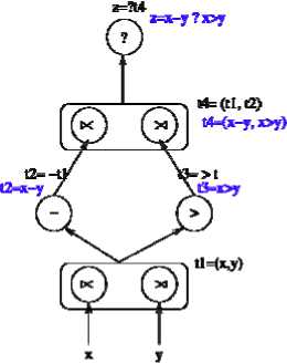
Figure 1:Graph of the expression z = x-y if x>y

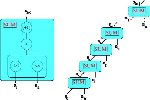
Figure 2: Graph of the expression

Table 6: Primitive expressions for expression fl =K 3 fl =x n 12 = +fl s= [+l]0 /2

relation s^tl пЛ ri 11412

where [+1] 0 indicates add one to index ze-ro. ¹

The expression is used to describe how iteration is achieved. Indices are introduced that do not have bounds. This expression is an infinite graph as shown in Figure 2.

An evaluation of these relations for s0=0, n0=3, n1=7 and n2=13 is shown in Table 7.

Table 7: Evaluation of Summation

Element	Expression	Result
3o =0 no =3 Ho = (0,3) i2o=3	t =x 3 f =x n 12 = +fl з = [+l]o 12	flo = O flo = 3, flo = (0,3) 12о = 3 3i =3
3t =3 m =7 Hi =(3,7) 12t =10	f =x з t =>« n 12 = +fl з = [+1 Io 12	Hi =3 Hr =7,11^ (3,7) 12, = 10 32 = 10
32 = 10 „2 = 13 H2 = (10.13) 122=23	t =K s 1 =x n 12 = +fl з = [+l]o <2	fl2= 10 fl2= 13,H2 = (10,13) 122 = 23 зэ=23

The Figure 3 shows the structure of a simple implementation of the model consisting of one processor. This implementation consists of: a queue of unprocessed elements that are waiting to be processed, the table relations and hash table. Elements are popped off the queue, processed using the relations – where the relation has a tuple operation the tuple is formed using the hash table, and finally the newly created elements are added to the queue.

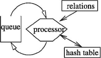
Figure 3: Structure of Element Model

The processor takes elements off the queue and loops through the relations indexed by the element name. The processor applies the operation in each relation to the values of the element. If the operation is defined, a new element is created with the range element name in the relation and the values or indices resulting from applying the operation. The newly created element is pushed onto the stack. The process continues until there are no more elements to process.

There are three classes of operations: those that result in a new value being computed; those that result in a new index being computed and those that compute a tuple. The paper does not go into the detail of all these operations. The only one requiring a little more detail are the operations that create tuples. The two elements used to create a tuple can come in any order. The first to arrive of the two elements that form a tuple is inserted in the hash table. The second element to arrive is then matched and the tuple is formed. The element name and the indices are used to match the two elements that form the tuple.

The model is inherently parallel as any processor that has the relations to process that element can process any element2. Thus the element in the unprocessed queue can be distributed across any number of processors.

• B.    Comparison with other architectures

The element-based architecture has no instructions. The only other models that do not use instructions are theoretical models like the Turing Machine. Data-flow architectures do not have instructions executed in a sequential order like the von Neumann. However, the nodes are typically referred to as firing instructions. Even so, data-flow architectures come close in terms of shifting the emphasis from executing instructions to processing data[6,7,8].

As with data-flow, element-based model programs can be viewed as graphs. The big difference is that the data-flow graphs are finite and allow for cycles, whereas in the element model programs, the graphs can be infinite and acyclic. A data-flow program is stored as a graph with pointers to the nodes in memory, restricting the graph to being finite and thus cyclic. A data-flow program cannot be represented by an infinite graph as can be done with the element-based approach. The element model achieves this by expressing the graph using classes of relations that represent infinitely many nodes and edges and not representing the graph as nodes and pointers in memory.

The unique aspect of this model is that values are not referenced by memory addresses, but rather, the semantic information required to process the elements is kept together with values. The processor determines how to process the value based on the element name and indices. In the von Neumann model it is an instruction that determines how the value will be processed. In the data-flow it is the instruction that gets fired when the required values arrive at a node.

Like the von Neumann model, the element model has a simple three step execution cycle but instead of executing the next instruction, the next element on the queue is processed. There is no concept of the program counter and hence the state of the program execution is determined by active elements that are on the queue of elements waiting to be processed. This contrasts with the von Neumann model, where the program counter and the contents of memory capture the state, or the data-flow model where the state is determined by the state of the nodes.

The data-flow model allows for parallelism in that any number of nodes can fire simultaneously. However there are a number of limitations. The cycles in the graph limit the degree to which available values can be processed. Either starting the next cycle has to wait for the previous cycle to finish or there has to be some mechanism for differentiating between cycles. The nodes are stored in memory that restricts the evaluation of values to take place in the processor where the nodes are stored. The element model is able to process all the active elements in any order and any number at the same time, limited only by the number of processors.

Being able to process elements in this way facilitates parallelism for a number of reasons. Processing an element is independent of other active elements and hence of the state of the program, thus any processor that has access to the relations associated with an element can process that element. The exception is forming tuples that requires a mechanism to handle that the two components of the tuple need to access the same hash table. It does come at a cost and that is an aspect that this research attempts to evaluate.

The element model is a functional one, yet different from current models. Instead of expressing and evaluating a program as a function that gets applied to values, a program is a set of algebraic expressions of relations between sets of elements. Such a relation defines the mapping between the elements of the two sets. A relation and an element in its domain are used to create an element in the range. Thus a relation, such as a = f(b), (5)

and an element in the domain, e.g.

b=(5,3), (6)

are enough to determine the element a=8. (7)

An element consists of an identifier (name and indices) and a value. The element name is used to establish for which relations the element is a member of its domain. When a new element is created, the relation determines what the identifier is and what operation has to be applied to determine the value of the new element.

Identifiers are used in a different way. Most languages typically express a function such as square something like square(x) = x*x .

In this example the variable identifier x has no significance other than that it represents the value passed to the function. The variable x can be used in the definition of other functions and using the same variable does not imply any relationship between these functions and the function square. An element example of a relation is volume = area * height. (8)

Here the meaning of area is not confined to this relationship. Hence using the same identifier in another relation relates the two relations. For example if there is another relation area = length * breadth,

then area refers to the same entity in both relations. Whereas the functional approach sees the function square as the mapping

RxR^R, the element-based relation describing volume is viewed as the mapping

.

The variable x has no significance once the function square has been computed. The element area has a life independent of the relation that created it and its meaning holds for the entire computation.

Since the meaning of an element holds for the entire computation, the order in which it is processed is not important. This property enables elements to be processed in any order as well as on different processors, facilitating parallel processing. This property also helps with programming. The programmer does not need to have to design the order in which the execution takes place and, more important, does not need to design the coordination between the processors. Since the meanings of elements are static, relations also are. This is unlike instruction-based programming where the programmer needs to take into account that a statement has different meanings as different values are iterated through it.

Given that in any program one is limited to a finite number of identifiers, this suggests that one is limited to a fixed number of elements and computations. Both instructional and functional models get around this by reusing identifiers. The element-based model overcomes this limitation by having element identifiers consisting of a name and indices. For practical purposes, this enables infinitely many unique element identifiers. By using implied universal quantifiers this enables any algebraic expression, such as si+1 = si + ni, (11) to define infinitely many relations, called a class relation, and to be able to process an unlimited number of elements. The name part of the identifier identifies the class relation and the indices instantiate a particular relation to process that element.

The element-based approach does not use indices in the same way as the instruction-based model. An index is part of the element identifier and not an offset into some fixed memory. The element name and indices provide the semantic information required to process the element and thus this avoids having to use addressing to access data. The other advantage is that elements are never altered: they are created, processed and discarded; hence there are no cache memory writes. Again this facilitates distribution across processors.

The element model is computationally equivalent to the instruction model as it can implement a Turing machine. A series of examples, such as sorts and pattern matching, have been successfully implemented. Like with any model some algorithms are better suited to the element model. The purpose of this research is to explore how the element model is likely to perform for the specific case of simple matrix multiplication. The reason this case has been chosen is that it is a tightly coupled computationally intensive example.

• III.    Research Approach

What is the best way to evaluate the proposed model, especially only having von Neumann hardware available? The success of the model depends on it being able to compete head on with current technology. For this reason, the choice was made to do a direct comparison with the instruction-based model. Since the research is around finding better models for parallel computing, the case study needs to focus on this aspect. Experiments were run on a cluster as this was the only resource available. An MPI emulation was used for running the element based programs. A comparison is made between a MPI C program and an element-based program.

The model is evaluated in 3 ways: ease of programming; use of resources; and performance. The evaluation of the model is done on a number of levels. An important one is how easy it is to write programs. As the language has not been discussed in detail, a brief comparison is given. The next level is a complexity analysis of the resources required, looking at memory requirements and number of instructions executed and how this scales with the number of processors. Data collected in the emulation of the element-based model is used to verify the analysis. Finally a study is made of how the runtimes of the two programs compare as the size of the matrix and the number of processors increases.

At the end of the day what matters is whether the element-based model has the potential to out-perform the current technologies, and in particular, scale better with the number of processors.

• A. The programs

To make a fair comparison and facilitate the analysis, the approach was to use the most basic design of the program for both cases. The algorithm for matrix multiplication of A = BxC is simple:

Ik-1

Vr € [0, n_r - 1], с e [0, л_Е - 1], Л_Г1С - B„t * C^ k=O

where n_c and n_r are the number of columns and rows.

This can be expressed as a simple C program as follows:

for (row-0: row «NoRows :row++)

I for(co1=0; col «NoCols; col-n-)|

A[row I [ col 1=0;

for ( k=0;k

A[row)[colJ += B[rowJ[k] • C[k][colJl

• Figure 4:    C Matrix Multiplication Code

In the case of the element base program one can almost use the expression as is. However to make the program more explicit we expand the above expression to:

Vre [0,»,-I]

Vee[0,»c-l]

^ - Еь»^, * C,*,

Vte[0,nc-l] B_r,_x = B„

Vke[0,n,-l] Ct„ = C,, and further develop it to:

^ = 4,16 11*1; q„ = C„ie |1тЯг]

>1rttr = BcU*C«U A^ = °

The “assembly” code is given in Figure 4.

H master for(row=0; row «NoRew: row -H-)

for(col=0; col send) nextproc ,B[row) ,C[col J);

receive (proc ,A[row ,col ]);

// slave receive (master , В, C);

result =O for(k=D; k

send (master, result);

• Figure 5:    MPI C Matrix Multiplication Code

The implementation of this is somewhat more complicated using MPI. Managing the slaves and synchronizing requires additional code provided in Figure 6.

The element-based program, by comparison, is inherently parallel and does not need to be rewritten to run on a parallel architecture. Also there are no built in restrictions as to the size of the buffers for message passing. Using an old measure of lines of code, the element-based program is a fraction of the size. There is no need to come to grips with message passing or synchronization. Not having to manage the parallelism gives the element-based approach an advantage.

From	To	Op	Index I	Valuev
b	bSO	xins	2	n-I
b$0	b$2	xnfltr	2	0
	a$0	tuple 0
b$2	b$0	xsub	2	1
c	c$0	xins	0	n-t
c$0	c$2	xnfltr	0	0
	a$0	tuple 1
c$2	c$0	xsub	0	1
a$0	a$l	mull
a$l	a$2	xfltr	1	n-I
	a$3	xnfltr	1	n-t
a$2	a$4	xsub	1	i
a$3	a$5	tuple 0
a$4	a$5	tuple 1
a$5	a$6	add
a$6	a$7	xfltr	1	0
	a$2	xnfltr	1	0
a$7	a	.vdel	1	1
a	print	print
Wlists

Op    Description int niainfint argc , char *argv[J)

{                                                                             "

int slave, noslavcs , result [4];

MPI-Status status:

M Pl -Сошли .rank ( MPLCOMM_WCK1D. & s 1 a vc );

MP1 -Comm-stze(MPI-OCMM-WlORLD. &bos laves):

^=------------------

H master slave

================= i f ( si a ve=m aster-8 lave)

int sizeM;

scamf(”%d”.&sizcM };

int A[ sizeM J [ sizeM] . В [ sizeM ][ sizeM ],

C[ sizeM ][sizeM] , row, col , re su It [ 5] ;

MPI-Status status:

//=========

// read in data

//========= for (row =0; row

for (col =0; colcsizcM: col 4-+)

MPLRccv( result , 5, MPIJNT, MPLANY^SOUKCE.

if (result []]! = -!)

A[ result [I ]][ result [2]]= result [3];

result [l] = row;

result [2] = eol ;

result [3]=0;

result [4]= sizeM:

resin .MHJDOMM-WOttLD);

nnvin ,MfWaMM_WORLt>):

colm .MHJ30MM-W0RLI>):

for(row=D; row

A[ result [1 ]][ re suit [2]]= result [3];

result [l]= -I;

) //end Maarcr

// ^==

// slave

// ==== else int B[100], C[100], result [5], i;

result [I]= -1;

result [0]= slave:

resin .MPIjDOMM-WOSLD );

while (1)

MPIJ1KV( result . 5. MPIJNT. 9.ream,

MPL£OMM-WORLa& status);

if ( result []]==-!) break ;

MPI-Rccv

rawin . MFICOMM-WORLD, & s t a t u s );

MPI-Recv(C, result [4], MPIJNT, 0, col in . MPtmVlMWGRLD As t a t u s );

result 13 ]=0:

for (i =O;i

result[3]*=B[ihC[il;

MPl-SeudfSrrcsulT , 5, MPIJNT, 0.

resin .MH-CQMM-WORLD);

) //end slave

MPl-Fiualizc ();

• Figure 6:    Parallel MPI Matrix Multiplication Program

The assembly code generated by the parallel version of the C program ran to 600 odd lines and 20 lines for the slave. A small sample is given in Figure 7. Comparing the element-based code with the C code, there is a close mapping between the element program and the low level machine code, in contrast to the instruction-based. In the element-based model the semantic gap between the high-level program and the machine code is small re- sulting in a small amount of machine code. The second aspect is that the element-based program does not need to be altered to run on a parallel architecture. It is inherently parallel.

1 awl $1M, -52(Xrbp)

2 жя1 -5206*p). Xedx

• 3    eorslq ledx.Xrax

• 4    salq $2. Xrax

• 5    ecwq Xrax, -12WI(Xrbp)

• 6    wwl -S2(Xrfap), %eai

• 7    BOTslq Kedx.Wrdx

I cltq

• 9    iealq Krdx, Xrax

It  salq   $2. Xrax

• 11  addq   $15. Xrax

• 12  addq   $15. Xrax

• 13  shrq   $4, Xrax

• 14  salq   $4, Xrax

• 15    subq Xrax, Xrsp

  16 leaq 16(Xrsp), Xrex

  17 eovq Xrex. -119206rbp)

  U eovq -1192O6*p). Xrax

  19 addq $15. Xrax

  2i shrq $4, Xrax

  21 salq $4, Xrax

  22 eovq Xrax, 1192CXrbp)

  23 eovq 11920Mp), Xrax

  24 eovq Xrax. 168(Xrbp)

  25 enel -52OMp). led*

  26 ami Xrdx. -llM($rbp)

  27 emrslq -ll»(Xrhp).Xrax

  28 salq $2, Xrax

  29 eorq Xrax, -1176(Xrbp)

  39 xml S2(Xrbp), Xeax

  
  

Figure 7: Sample of assembly code for MPI program

• B.    Complexity Analysis

The complexity of the instruction-based model can be measured in terms of the number of instructions, whereas for the element-based model, elements can be used. A starting point is to show that the complexity of the element-based model is at least equivalent, if not better, than the instruction-based model for the matrix example. Having established that the complexity of the element-based model is comparable with the instruction model, the focus can turn to a comparison between the execution times and scalability with increased number of processors.

The analysis is a waste of time if processing an element is clearly vastly more expensive than executing an instruction. On the basis of the instruction cycle versus the element cycle, creating an element is argued to be at least as efficient as processing an element. Consider each step in the cycle.

Accessing/storing elements from/to hardware queues should give the element-based approach a major advantage over having to read/write data from/to memory. The element-based approach has the potential of being able to delay paging to access relations until there is enough demand. Except for tuples, information is only read, eliminating the need for cache block write-back. Any number of elements can be processed in parallel, as there are no dependencies between them. This scaling factor has the potential to far exceed any pipelining approach of the instruction model. Even though it is not clear what the full cost of performing the tuple operation will be, this seems a reasonable initial assumption that the cost of creating an element is likely to be better than performing an instruction.

Table 8: Comparison of memory accesses

Step 1 2 3 4	Instruction-based	Element-based
	get instruction	pop element
	memory access	stack register
	cache/page faults	none
	get data	get relation
	memory/register	memory
	cache/page faults	cache/page faults
	perform instruction	evaluate relation
	exception branch inst	exception tuple op
	cache/page fault	cache/page fault
	store	push element
	memory/register	stack register
	cache/page faults	none

For the analysis, the multiplications of лхл matrices are compared. The master has an outer loop of 97 instructions and the inner loop is 92. The slave has 79 instructions of which 27 are in the loop. Every time the slave is passed a message it loops n times to compute one element in the resulting matrix resulting in 27n instructions. For every entity in the resulting matrix, a message is sent to the slave that is n² messages. Thus, the number of instructions computed in the slave's loop is 27n³. There are 52 instructions remaining in the slave if one excludes the instructions in the slave's loop and the 92 instructions in the inner loop of the master that are executed for each row and column. This gives 144 instructions that are executed n² times. There are 5 instructions in the outer master loop not in the inner loop that are executed n times and some constant c instructions that are only executed once in the master. Thus the number of instructions executed for a л x л matrix is 27n³+144n²+5n+c. This ignores the cost of the calls to MPI subroutines that should result in a significant number of additional instructions that get executed.

Table 9 works out the number of elements processed to be 14n³+7n². It should be no surprise that the number of instruction/operations in both the instruction and element-based programs are of order n³. Even so the number of elements processed, 14n³+7n², is more or less half the number of instructions executed by the instruction-based program, 27n³+144n²+5n+c. However, the real issue is what improved performance can be expected by increasing the number of slaves and how the speed scales with increasing number of processors.

Consider the instruction-based C program first. Given m slaves, the calculation of n2 entries of the resulting matrix is distributed to the m3 slaves as these processors become available. Given an ideal environment, in which there are no delays in sending and receiving data, the speed up should be directly related to the number of processors. The purpose of the empirical study is to assess

• •    what the overhead of the MPI model is on achieving this as well as the cost of transferring the data and

• •    the weaknesses the instruction-based model has i.e. the memory wall, page faults etc.

The particular program that is used does have a limit on the size of the matrices it can handle. Other aspects that affect the performance are cache faults that can only be measured empirically.

Table 9: Analysis of Elements Processed

domain     range      op			number
	b		2 n
	c		2 n
b	b$0	xins	n2
b$0	b$2	xnfltr	n3
	a$0	tuple 0	n3
b$2	b$0	xsub	n3
c	c$0	xins	n2
c$0	c$2	xins	n3
	a$0	tuple 1	n3
c$2	c$0	xsub	n3
a$0	a$1	mult	n3
a$1	a$2	xfltr	n3
	a$3	xnfltr	n3
a$2	a$4	xsub	n3
a$3	a$5	tuple 0	n3
a$4	a$5	tuple 1	n3
a$5	a$6	add	n3
a$6	a$7	xfltr	n3
	a$2	xnfltr	n3
a$7	a	zdel	n2
a	print	print	n2
			14n3+7n2

• C.    Empirical Study

In the previous section a case is made that, potentially, the element model has significant advantages over the instruction model. However the argument is based on a number of assumptions. This section tries to get some handle on how valid these assumptions are. The runtimes of the instruction-based and the element-based programs are collected for different sizes of matrices and different numbers of processors. These runtimes are compared to assess:

• •    whether the element-based program execution times are comparable with the instruction-based execution times, given that the code is emulated on an instruction-based computer, and

• •    whether the element-based model scales better with the number of processors.

An MPI program (see Figure 8) was used to emulate the behavior of the model to give some idea of its possible performance and highlight weaknesses. The results give some indication of the potential performance of an element-based architecture. An evaluation of the experiments is used to assess the validity of the assumptions made in the complexity analysis. On the basis of these results an assessment is made as to whether the element model is worth investigating further.

Experiments were undertaken to assess if there are grounds to support the arguments that an element-based model:

• •    can be implemented to do a computation such as matrix multiplication,

• •    performs better without parallelism, and

• •    scales better with increasing number of processors.

The experiments involve comparing the performance of the emulation of the element-based program and the execution of the C program. The following data is compared:

• •    the number of elements created with increasing sizes of matrices with a single slave,

• •    the wall times of both with increasing sizes of matrices with a single processor, and

• •    the wall times of both for a given size of matrix with increasing number of slaves.

The simple emulator shows that it is possible to implement the model of computation to compute problems such as matrix multiplication. The model does handle the essential primitives i.e. selection, iteration and progres-sion4.

The predicted number of elements relates closely to the number of elements processed. The difference with the analysis 14n³+7n² differs by a factor of n² shown by Table 10.

Table 10: Comparison Between Predicted and Actual

Size Predicted            Actual

100	14 070 000,00 14 960 000,00
110	18 718 700,00 19 916 600,00
120	24 292 800,00 25 862 400,00
130	30 876 300,00 32 887 400,00
140	38 553 200,00 41 081 600,00
150	47 407 500,00 50 535 000,00

One reason for the discrepancy is an implementation design aspect that results in an additional element being created for each tuple operation. This is not a significant difference and aspects like system calls by the C program can result in similar discrepancies. This result supports the argument that the element-based model will perform better, given the assumption that creating an element is no worse than executing an instruction.

If we look at the execution times for the matrix of 100 by 100 in Table 11 we see that the number of instructions per time unit is 15.5 for the element based technique and 240.8 for the instruction based one. This is roughly 15.5 times slower than the C program. Considering that the emulator has to execute well over twenty instructions for processing each element, it suggests that the assumption, that processing an element is at least equivalent to processing an instruction, may be a reasonable one. If one takes into account that the estimated number of instructions executed is three times the number of elements evaluated, this reduces the gap to just over 5 times slower.

while (I stackEmpty )

( pop (element);

new.element=elemenl;

next Relation— relationTable [element. id ]. Li s t ; numberRelations = relationTable [element. id ]. size ;

for(i=0; i

I new-element. id — relation [nextRelation]. id ;

case ( rel ation [ next Relation ]. op)

H arithmetic and logical operations add:

( new.element. value [0] += element. value [1]; break:

// index operations indexAdd:

I new-clcmcnt. index[ relation [nextRelation ],parm0]] += relation [nextRelation].patml I;

break;

}

// if operation ifop :

I if (! new-element. value [I])

goto skip: // do not create a new element break;

joint:

int found;

checkHashTable(newElement, found); if (! found) goto skip;

break;

J processSlave= slave.mapping(ncwHlcmcnt. index , noslaves ); push(processslave .newElement);

skip :

I

I

Figure 8: Outline of Emulator

The picture does not look so favorable when the matrix size increases and the element-based model is from 5 times for (100 by 100) to 7.5 times slower for (150 by 150) see Table 11. However the emulation is at present a very simple implementation and on a totally unsuitable architecture. Like with the current architectures, considerable effort will need to be put into its design. Since elements do not need to be processed in a predetermined order, this enables the processor to better manage the resources by determining the order in which elements are processed. This could have significant impacts on the implementation of the tuple operations that could explain the deterioration of performance as the size of the matrices increase.

The next comparison given in Table 11 looks at how the two approaches speed up with the number of slaves. The instruction-based times do not improve beyond two slaves whereas we see that the times of the element-based program do. The execution times for the element-based program show some unexpected results, even though for all measures, the best wall time of five executions was selected. Part of the problem may be a property of the cluster. Both the instruction and element-based times seem out of line for the case with 6 slaves. The picture looks much better for the element-based program if we look at the speedup factor. The performance is better than linear up to 8 slaves and unexpectedly there is a degree of superscalar speedup. This result further supports the argument that this model needs to be explored further.

Table 11: Comparison of wall times

Size	Element-based		Instruction-based
	Predicted	Time	Predicted	Time
100	14070	907	42141	175
110	18719	1211	56072	280
120	24293	1530	72778	322
130	30876	2052	92511	398
140	38553	2665	115523	410
150	47408	3299	142066	442

Table 12: Comparison of wall times

Number Processors	Elem Time	Speed up	Instr Time
1	10207	1.0	978
2	3959	2.6	646
3	3315	3.1	627
4	2250	4.5	573
5	1728	5.9	672
6	1865	5.5	661
7	1193	8.6	620
8	1198	8.5	626

IV. Evaluation and Conclusion

This paper presents an alternative computational model that has significant advantages. The most significant is the concept of processing elements one at a time in a similar way to processing instructions. Underpinning this mechanism is that elements encapsulate both semantic information and data. The semantic information is used to determine how an element gets processed to create new elements. Like the von Neumann model, the evaluation cycle is a simple three-step process.

Since this paper is focused on the model as the basis for parallel architectures, the description of programs is touched on. The program in the case study is expressed in basic algebraic notation that maps closely to the machine level code. There is a small semantic gap between the program and the code, unlike the C program. Both the source and the assembly code are more concise than the equivalent C program. The element program has a big advantage in that it is inherently parallel and does not need to be specially designed for parallel processors. If the case study is representative of writing programs for parallel architectures, then the element base architecture has a decided advantage.

The complexity analysis of the two programs unsurprisingly shows that both are of order n³. However, on the basis of the given assumptions and potential advantages of the element-based model, the analysis indicates that the element-based model is more efficient than instruction-based model. Both programs should exhibit linear speedup with the number of processors.

The element-based execution times were considerably better than was expected, given that the element-based execution used a crude emulator running on an instruction-based cluster. The area of concern is around the decline in performance as the matrix size increases. The suspected reason for this is the hashing with the associated page faults. More investigation is needed to explore how to improve the tuple hashing by ordering the processing of tuples. Being able to use hardware queues rather than addressed memory access for the unprocessed elements, as well as passing elements between processes, should further improve the performance.

The element-based execution times showed a better than linear speedup whereas the instruction-based did not. This contradicts the complexity analysis for the instruction base model that it would. This provides the strongest case that the element-based model may be a better model for parallel architectures.

This paper provides evidence that, for a tightly coupled memory intensive program, the element-based model has the potential to perform better than the instruction-based model. The next step is to implement the model using FPGAs [9]. However this is beyond my resources without some support for the potential of the model. Research is continuing informally, describing both the theory underpinning the model and the language.