Energy circuit of a thermal circuit with a direct-acting regulator with a capacity of 1 MW in pulsating mode

Бюллетень науки и практики / Bulletin of Science and Practice

UDC 621.316.728                                   

The energy circuit of a thermal system represents a crucial aspect of its operation, dictating the flow and distribution of energy within the system. In the context of thermal circuits employing direct-acting regulators, ensuring optimal energy management becomes paramount, particularly in scenarios characterized by pulsating modes of operation. This introduction delves into the intricacies of energy circulation within a thermal circuit featuring a direct-acting regulator with a

(ос) ® capacity of 1 MW operating in pulsating mode. By elucidating the interplay between energy input, regulation, and output, this discussion aims to shed light on the challenges and opportunities inherent in such systems. Through a comprehensive examination of the energy circuit dynamics and the role of the direct-acting regulator, this study endeavors to propose innovative solutions for enhancing system performance, efficiency, and reliability. The environment is very important [1].

In 2018, Xu [2] used a steam generator simulator to study the unsteady pressure pulsation characteristics of the reactor coolant pump at different flow rates and different rotational speeds. They used fast Fourier [3-11] transform and root mean square methods to analyze the pressure pulsation signals measured by sensors on the pump casing and oil outlet pipe. Under different flow rates, the pressure amplitude of FRPF increases with the increase of rotation speed, but the pressure amplitudes of FR and FSPF fluctuate slightly with the increase of rotation speed. Zhang [12] employed CFD numerical simulation to investigate the mechanics of non-uniform flow within the channel-head of the SG and discovered that the channel-head’s asymmetric structure and the abrupt contraction of the connection between the channel-head and the inlet pipeline caused flow separation, resulting in non-uniform inflow.In 2024, Zhang [13] took the third-generation reactor RCP as the research object and used CFD to study the unsteady characteristics of the third-generation RCP under non-uniform inflow conditions, focusing on the pressure pulsation characteristics inside the RCP. It was found that non-uniform inflow can cause unstable pressure fluctuations in the "throat" area of the channel head.

The principle of operation of the experimental setup. Figure 1 shows an experimental setup for the ITP coolant supply regulator.

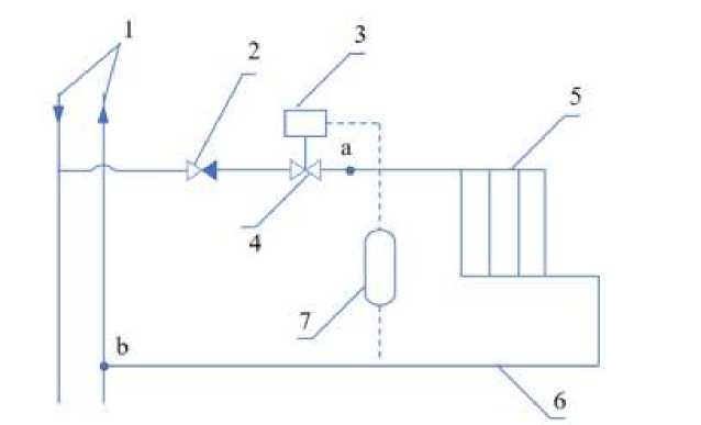
Figure 1. Experimental setup for the ITP coolant supply regulator: 1 – heating network; 2 – check valve; 3 – regulator; 4 – valve; 5 – heating devices; 6 – pipeline; 7 – sensor

Thermal energy comes from the heat network 1. The amount of thermal energy is regulated by the regulator 3, by a signed from the sensor 7. When the valve of the regulator 3 is closed, the flow rate and pressure on the heating device 5 will drop. Since the ambient air temperature is constantly changing, the regulator 3 always work.

In the course of the study, for a better understanding of the scheme, it was decided to study 2 characteristics of hydraulic and thermal, in order to better understand the nature of the forces arising and to more accurately determine the required parameters on the obtained model.

In the first power circuit the hydraulic characteristics at the moment of closing of the shock valve is considered. This circuit contains 3 elements.

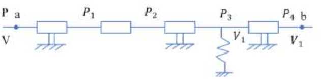
Figure 2. Hydraulic circuit

The circuit link equations:

ГР = Г1У2+тУ+ т2У2+Т3У12+ Р4

(          У = /Р з + У 1

Equations for Р₄,Р₃,Р₂,Р 1 :

Р4 = Р40 + Р4

Рз=ГзУ12+Р4(3)

Р2=ЪУ2+Рз(4)

Р^тУ + Р2(5)

Equations for У 1 :

у = У10 + У у2 = У2, + 2У1оУ

Equation for Р3, Р3:

Рз = Г3У2 + Р4=Г3 У12о + 2Г3У10У + Р40 + Р4(8)

Р3 = 2Г3УЮУ + Р4

Equation for Р2:

Р2 = Г2У2 + Г3У120 + 2Г3 710^1 + Р40 + Р

Equation for Р 1 :

Р1 = тУ + г2У2+г3У20 + 2г3У10У1 + Р40+Р4

Equation for Р:

Р = 01 + т2)У2 + тУ + г3У20 + 2г3У10У, + Р40 + Р4

Equation for У:

У = 1Р3 + 71 = 21г3У10У1 + 1Р4 + У10 + 71

Equation for У:

У = 2/г3У10У1 + 1Р4 + У

Equation for У2:

V2 = (V10 + 2lr3V10V1 + /Р4 + У1)2 = У102 + 4У102/г3У1 + 4У10/Р4 + 4У10У1

Equation for Р:

Р = (п + г₂)(7ю² + 47 ioWi + 4V_wlP 4 + 4VM + m^V^ + IP 4 + V i )

^{+ r}3^V2o ^{+ 2r}3^Vio^Vi

Equation for images:

(« i s + a 2 )V i (s) = -(b i s² + ^b2 s)P₄(s)                             (17)

Coefficients:

^ai = 2 ^lr3^Vio

« 2 = 1

b1 = ml b2 = 4l^2Vio

Complex circuit resistance Z (s) :

^p4⁽ s) _   a i S + « 2

^(S) = V i (s) = —(b i S²+b 2 S)

Frequency function of the circuit:

s ^ №>j² = —1

Frequency function of the circuit:

a i jQ+a2  _  (a i jn + a2^(b i n² + b 2 jn)

^Z( ) b_iQ²—b₂jft   (b_ift² — b₂j^)(b_i^² + ^b2 j^)

(aibijft3 — aib2ft2 + a2bift2 + a2b2jft)

=           b2^4 + b22n2

The real part of the frequency function:

—a b?Q2 + a?b ft2 Re(jO) =  ^----2t^~ b2Q4 + b22n2

Imaginary part of the frequency function:

^a i ^b i^³ + 0^2^ .

^,mW =^ft 4+^^j

Amplitude-frequency response (frequency response) of the circuit:

AW) = jReWy+lmW)²                      (24)

Phase frequency response (FFC) of the circuit:

imW) ?№) = -arctg-^

Calculate heat transfer energy circuit.

t_____ 11 ti ti r: t:__ t* ; 13 t q ~ l q qi _ _ «в <|2     _ q

Сз

Figure 3. Heat transfer energy circuit

The circuit link equations:

Ct = r1q + r2q! + r3q2 + t3

( q = c1t1 + c2t2 + q2

Equations for t3,t2,t2,ti,q2:

^t3 = ^t 30 ^{+ t} 3

t2 = r3q2 + t3

t2 = t2 = r3^2 + t3

ti = Wi + t2

^q2 = ^q20 ^{+ q}2

Equations on q1from the 1st link:

^q 1 = ^c2^t2 ^{+ q}2 = ^c2^(r3^q2 ⁺ ^ 3 ) ^{+ q}20 ^{+ q}2 = ^c2^r3^q2 ^{+ c}2^t3 ^{+ q}20 ^{+ q}2

Equations on t₂ from the 1st link:

t2 = ГзЯ2 + t3 = ГзЯ20 + ГзЯ2 + *з0 + t3

The equation on t_i :

t1 = r2qi + t2= r2(c2T3q2 + c2t3 + q20 + q2^ + (^q + T3q2 + t30 + Ц) = c2r2r3q2 + (r2 + r3)q2 + (r + r^o + c2r2t3 + t3 + t30

The equation on t_i :

ti = c2r2r3q2 + (r2 + r3)q2 + c2r2t2 + t3

The equation on q :

q = citi + c2t2 + q2

= ci [c2T2r3q2 + (r2 + r3)q2 + c2r2t2 + t3] + c2(r3q2 + t3) + (q20 + q2)

= c^rrq? + (c^ + cir + c2r3)q2 + q2 + q20 + ^2^2

+ (ci + c2')t3

The equation on t:

t = riq + r2qi + r3q2 + t3

= biq2 + Ь2(Ь+ b3q2 + b4q20 + a^ +a2t3 + a3t3 + a4t3Q

Equation for images:

(ais2 + a2S + a^Q^s) = -(bis2 + b2S + b3)T3(s)

Coefficients:

ai = cic2rir2 a2 = ciri + c2ri + c2r2

a3 = 1 bi = cic2rir2r3 b2 = cirir2 + cirir3 + c2rir3 + c2r2r3

^ 3 = ? 1 + ?2 + Г з

Complex resistance Z (s) :

T(s) a s2 + a2s + a3 2

()   Q2(s)   —b1s2 — b2s — b3

Frequency function of the circuit:

s ^ \^,j2 = —1

Frequency function of the circuit:

Z(s) =

T3(s)    a1s2 + a2s + a3

—a1^2 + a2\Q + a3

Q2(s} —b1s2—b2s — b3    Ь1^2 — Ь2)^ — Ьз

——a1b1^4 + О1Ьз^2 —

a2b 2112 + a3b1^2 — a3b3 + (a2b1^3 a2^3^^ + a3b2^)j

— a^ft³]

(b1^2-b3)2 + b^2

We derive the real part of the complex resistance:

Re(j 12) =

—a1b1^4 + a1b3^2 — a2b2^2 + a3b1^2 — a3b3

(b^—by + b2^2

We derive the imaginary part of the complex resistance:

(a b П3

Im(jO) = - 2 1

— a1b2^ —

о^Ьз^ + ОзЬ2^)

(b1^2-b3)2 + bl^2

We obtain the amplitude-frequency function of the energy circuit:

A(jO) = ^Re(jO)2 + Im(jO)2

Get the phase-frequency function of the energy circuit:

Im(jH')

MV = -arctg-^)

Construction of frequency characteristics of the circuit when changing at least three

parameters. Parameter are calculated or found from the experiment. Are set by the input power of the circuit, n₀ = 60 W, as well as the inlet pressure P ₀ = 300 kPa. Hire the pressure loss on the active resistance is assumed 5 ± 10%.

V =^. = -6L= 0.2l/s 0   P0   300       1

According to equation write the formula for r 1 , r₂r₃:

P0 * 0.1   0.1 x 300

Г = ---7

¹       v²

0.22

Г2 = 2r1;

г3 = 4r1;

Г kPa • s²l = ⁷⁵⁰ hH

The mass of water depends on the volume of pipelines.

m = 15 kg

Бюллетень науки и практики / Bulletin of Science and Practice Т. 10. №6. 2024

The compliance is found for equation: Vo * 0.5   0.2 * 0.5 I = —■---=      тг; = 0.0011 Po * 0.3   300 * 0.3 Algorithm for plotting graphs. CIRCUIT PARAM		Г lit • si L kPa J ETERS		(50) Table 1
m, kg	N       N       N Г 1’m-s      Г' 2 , m-s       r3 ,m.-s	l, lit • s/kpa	P o , kpa	V io ,lit/s
15	750        1500        3000	0,0011	300	0.2
30	750        1500        3000	0,0011	300	0.2
15	375         750        1500	0,0011	300	0.2

Dependency graphs are plotted based on the input values. For the best perception of graphs values are taken only those that affect the dependence. The values obtained for the first stage of the energy circuit are shown in Table 2.

Table 2 RECEIVED INFORMATION FOR HYDRAULIC

Ω	AjQ1	^j^1	Aj^2	^j^2	Aj^3	^j^3
1	1.2544	0.6608	1.2542	0.6733	1.8148	1.0124
2	1.8753	1.0336	1.9290	1.0765	3.3068	1.3139
3	2.7313	1.2337	2.9147	1.2965	5.0083	1.4453
4	3.7723	1.3528	4.0366	1.4214	6.6127	1.5194
5	4.9237	1.4291	4.9854	1.4948	7.6950	1.5658
6	6.0502	1.4801	5.4975	1.5388	8.0085	-1.5457
7	6.9850	1.5149	5.5499	1.5656	7.6781	-1.5261
8	7.6017	1.5392	5.2983	-1.5595	7.0118	-1.5137
9	7.8672	1.5562	4.9109	-1.5494	6.2597	-1.5059
10	7.8345	1.5682	4.4949	-1.5434	5.5515	-1.5015

Based on the results of the calculation, the graphs of the amplitude frequency response and phase-frequency response and frequency response of the circuit are constructed. Further in these graphs are under construction:

A

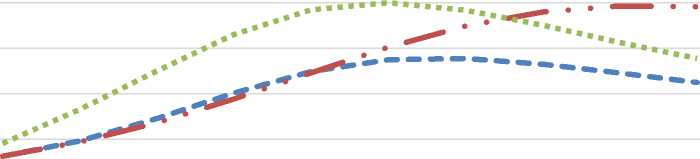
AjΩ1

AjΩ2

AjΩ3

1       2       3       4       5       6       7       8       9      10

Figure 4. Amplitude frequency response

1,5

0,5

-0,5

-1

-1,5

Φ

ΦjΩ1

ΦjΩ2

ΦjΩ3

-2

Figure 5. Phase frequency response

In the process of modeling the hydraulic power circuit, it is found that as the amplitude of the hydraulic circuit increases and the mass increases, the frequency decreases and then remains stable; as r decreases, the amplitude increases and the frequency decreases faster. The known conditions:

n_o = 15001^ t_o = 70% « 1 :800 - 1000 « 2 :10-15 F = 2m²,5 = 2mm

By calculation:

« 0

Qo= — to

w

21.429 У

1       1           kPa • s²

^Г 1 = « 1 F = 1 x 2 = ^{0.5 [} lit

0.002

m = — = -—-—-

2 AF 0.140 x 2

kPa • s²l = ^{7143 x 10 -3} hH

^3=4 « 2 ^F

0.010 x 2

kPa • s²l

=50hH

Aq Q-_Q1    2.14 ²⁹           г ^l

0.5to    0.5to    0.5 x 70    .     L • %

_c 2 = _C1 = 0.0612

^]

The limit of change Q is accept, Q = 1 . 10 rad/s.

Table 3

RECEIVED INFORMATION FOR HEAT TRANSFER

n0,kw	r 1 ,%2/w	r2,%2/w	r3,%2/w	c 1 ,w/%2	c2,w/%2	to, %	^w°c
1.5	0.5	7.143x 10-3	50	0,0612	0,0612	70	0.140
1.5	2	7.143x 10-3	50	0,0612	0,0612	70	0.140
1.5	4	7.143x 10-3	50	0,0612	0,0612	70	0.140

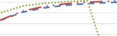
The dependency graph is drawn based on input values. For optimal graph perception, take only those values that affect dependencies. The obtained values for the first stage of heat transfer are shown in Table 4.

VALUE AMPLITUDE FREQUENCY RESPONSE FOR ENERGY CIRCUIT

Table 4

Ω	AjQ1	(pjH1	AjH2	(pjH2	AjH3	(pjH3
1	0.0198	-0.0006	0.0195	-0.0092	0.0196	-0.0327
2	0.0199	-0.0012	0.0203	-0.0169	0.0222	-0.0502
3	0.0199	-0.0018	0.0215	-0.0225	0.0253	-0.0544
4	0.0201	-0.0024	0.0230	-0.0258	0.0282	-0.0522
5	0.0203	-0.0029	0.0246	-0.0274	0.0306	-0.0480
6	0.0204	-0.0035	0.0261	-0.0278	0.0325	-0.0435
7	0.0207	-0.0039	0.0276	-0.0274	0.0339	-0.0394
8	0.0209	-0.0044	0.0289	-0.0265	0.0349	-0.0358
9	0.0212	-0.0048	0.0302	-0.0254	0.0358	-0.0327
10	0.0214	-0.0052	0.0313	-0.0243	0.0365	-0.0299

A

0,04

0,035

AjΩ1

AjΩ2

AjΩ3

0,03

0,025

0,02

0,015

0,01

0,005

1      2      3      4      5      6      7      8      9      10

Figure 6. Amplitude frequency response

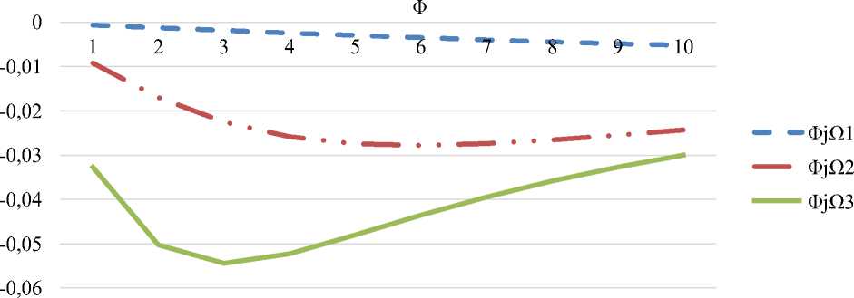
Figure 7. Phase frequency response

In the process of modeling the heat transfer process of the energy loop, it is found that the frequency response of the hydraulic loop decreases with increasing resistance and the amplitude increases.

Conclusion

In the course of the work, the problems associated with this work and possible solutions are described. A constructive scheme of the experimental device is proposed and the principle of its operation is described in detail. The power circuit of the device is drawn up, each link is explained. Complex impedance, frequency function, amplitude-frequency characteristic and phase-frequency characteristic are obtained by mathematical transformation of the power circuit. The frequency response of the circuit is constructed.

The description of the experimental setup is completed, energy circuits for hydraulics and heat transfer are compiled.

In the process of modeling the hydraulic power circuit, it is found that as the amplitude of the hydraulic circuit increases and the mass increases, the frequency decreases and then remains stable; as r decreases, the amplitude increases and the frequency decreases faster.

In the process of modeling the heat transfer process of the energy loop, it is found that the frequency response of the hydraulic loop decreases with increasing resistance and the amplitude increases.

According to the resulting graphs, one can trace the relationship between two different properties. It can be seen from the graph that for a particular r value, we reach the frequency maximum faster.