Enhanced Performance of Multi Class Classification of Anonymous Noisy Images

Published Online February 2014 in MECS

Multi class image classification is very important in image analysis. This plays an important role in many computer vision applications such as biomedical image processing, automated visual inspection, content based image retrieval, and remote sensing applications. Image classification algorithms can be designed by finding essential features which have strong discriminating power, and training the classifier to classify the image. Scientists and practitioners have made great efforts in developing advanced classification approaches and techniques for improving classification accuracy ([1],[ 2],[ 3],[ 4],[5], [6]).

A novel texture classification method via patchbased sparse texton learning is presented in [7].

Global image features are extracted for the purpose of texture classification using dominant neighborhood structure is proposed in [8]. Features obtained from the local binary patterns (LBPs) are then extracted in order to supply additional local texture features to the generated features from the dominant neighborhood structure.

Texture classification system based on Gray Level Co occurrence Matrix (GLCM) is presented in [9]. They have calculated GLCM from the original texture image and the differences calculated along the first non singleton dimension of the input texture image.

Different texture images are classified based on wavelet texture feature and neural network in [10].

The learning process is achieved through the modification of the connection weights between units. In the work [11] describes multi spectral classification of land-sat images using neural networks. The classification of multi spectral remote sensing data using a back propagation Neural network is presented in [12]. A comparison to conventional supervised classification by using minimal training set in Artificial Neural Network is given in [13]. Remotely sensed data by using Artificial Neural Network based have been classified in [14] on software package.

In this paper images of 16 classes are classified under different spatial conditions. Firstly they are classified without any noise; secondly they are classified under some unknown noise and lastly filtered through wiener filter.

This paper is organized into eight different sections including the current one. In the second section different statistical texture features are discussed. Section 3 is about noise detection in image and removal of noise with appropriate filtering method in section 4. Next is discussion about feed forward neural network in section 5. Section 6 is proposed methodology. Section 7, describes the experimental setup of the method. And the last one section 8 discusses the Implementation and result discussion.

• II.    STATISTICAL MOMENT FEATURES

Texture is a property that represents the surface and structure of an image. Generally speaking, Texture can be defined as a regular repetition of an element or pattern on a surface. Statistical methods analyze the spatial distribution of gray values, by computing local features at each point in the image, and deriving a set of statistics from the distributions of the local features [15].

Valavanis et al [16] proposed a system to evaluate the diagnostic contribution of various types of textures features which includes first order statistical moments feature in discrimination of hepatic tissue in abdominal non enhanced computed tomography images.

Depending on the statistical analysis of the image six features are extracted as follows:

• A.    Feature (1)

Mean or the average as described in (1).

1N xVZ (x - x)                       (1)

• B.    Feature (2)

The standard deviation: The best known measure of the spread of distribution is simple variance defined in (2).

var =

N - 1

n

Z ⁽ X - x) 2

I = 1

The standard deviation is a well known measure of deviation from its mean value and is defined in (3) as the square root of variance

CT =

var

• C.    Feature (3)

Smoothness is measured with its second moment as in given (4)

Smoothness = 1 -

(1 + var)

• D.    Feature (4)

The skewness, or third moment, is a measure of asymmetry of distribution given in (5).

skew = ^^= J* ; -*]³                    (5)

• E.    Feature (5)

Energy is statistical measure given in (6)

energy = ZZ P d ^{( i} , j)                  ⁽⁶⁾

ij

The gray level co-occurrence matrix P for displacement vector d=( d x , d y ) is defined in (7). The entry (i,j) for P_d is the number of occurrences of the pair of gray levels i,j which are distance d apart.

Pa ⁽ i ,j ) = |{((r,s),( t, v)y. I(r,s) = i, I( t, v) =

J ^}|                                                         (7)

• F.    Feature (6)

Entropy is calculated as given in the (8)

ij entropy = -ZZ Pd (i, j) log Pd (i, j)        (8)

ij

It should be noted that spatial gray level cooccurrence estimated image properties are related to the second order statistics of image. Thus six statistical texture features are calculated first for every image and then for every block of an image. The feature vector is populated with multiples of six with that of number of blocks in an image.

• III.    NOISE TYPE DETECTION

An image is often corrupted by noise in its acquisition or transmission. Noise is any undesired information that degrades the image and appears in images from a variety of sources. Basically, there are three standard noise models [17], which model the types of noise encountered in most images; they are additive noise, multiplicative noise and impulse noise. In this work we have considered the occurrence of additive noise .

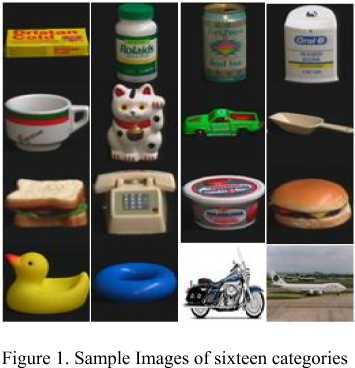
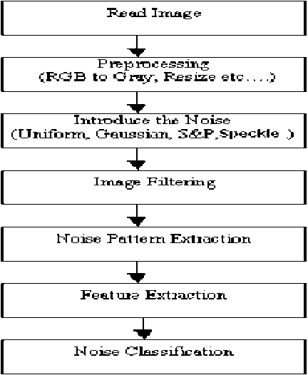
Figure 2. Block diagram of noise classification system [18]

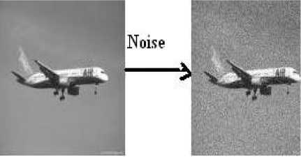
Figure 3. Original image affected by Gaussian noise

An image function is given by f (x, y) where (x, y) is spatial coordinate and f is intensity at point(x, y). Let f (x, y) be the original image, g(x, y) be the noisy version and η(x, y) be the noise function, which returns random values coming from an arbitrary distribution. Then the additive noise is given by the equation.

g(x, y)= f (x, y)+ n(x, y) (9)

Additive noise is independent of the pixel values in the original image. Typically η (x, y) is symmetric about zero. This has the effect of not altering the average brightness of the image. Additive noise is the good model for the thermal noise within photoelectric sensors.

In most of the research work of multiclass classification good images are taken for classification ([2],[3],[4],[14)]. Since noise affects the performance of features extracted for classification. Therefore it is necessary to remove noise from the images for classification. Scientist and researchers have rarely performed classification in noise constraints. Sometime images which are to be classified may contain noise also, but these are unknown. Then the result of filtering may not produce good quality image. So if we know which noise occurs in the image then appropriate filtering operation will give better noise removal.

Shamik et. al [18] has discussed a novel method of noise detection and classification. They have detected and classified four types of noise uniform noise, Gaussian noise, speckle noise and impulse noise as shown in the fig. 2.

In this research work, Gaussian noise pattern as shown in fig 3 is detected in our images based on methodology discussed in [18]. Where statistical moments features are extracted from the noise patterns for noise class detection. This experiment detects the Gaussian noise patterns from images. This leads to applying of wiener filter on noisy images, which gives the best noise removal.

• IV.    SPATIAL FILTERING

Noise having Gaussian-like distribution is very often encountered in acquired data. Gaussian noise is characterized by adding to each image pixel a value from a zero-mean Gaussian distribution. The zeromean property of the distribution allows such noise to be removed by locally averaging pixel values [19]. Conventional linear filters such as arithmetic mean filter and Gaussian filter smooth noises effectively but blur edges. Since the goal of the filtering action is to cancel noise while preserving the integrity of edge and detail information, nonlinear approaches generally provide more satisfactory results than linear techniques.

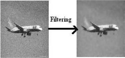
Figure 4. Applying Wiener Filter on noisy image

Wiener Filtering

Wiener filter estimates the local mean and variance around each pixel.

=    ∑   _,   ∈    (  ,   )

and

=   ∑      ∈     (  ,  )-   ,

,

Where is the N -by- M local neighborhood of each pixel in the image A. Pixel wise Wiener filtering using these estimates,

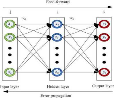
Figure 5. Feed Forward Back propagation Neural Network

(  ,  )=  +      ( (  ,  )- )            (12)

Where ν2 is the noise variance. If the noise variance is not given, wiener filter uses the average of all the local estimated variances.

• V.    NEURAL NETWORK AS CLASSIFIER

A successful pattern classification methodology [17] depends heavily on the particular choice of the features used by the classifier .The Back-Propagation is the best known and widely used learning algorithm in training multilayer feed forward neural networks. The feed forward neural net refer to the network consisting of a set of sensory units (source nodes) that constitute the input layer, one or more hidden layers of computation nodes, and an output layer of computation nodes. The input signal propagates through the network in a forward direction, from left to right and on a layer-bylayer basis. Back propagation is a multi-layer feed forward, supervised learning network based on gradient descent learning rule. This BPNN provides a computationally efficient method for changing the weights in feed forward network, with differentiable activation function units, to learn a training set of input-output data. Being a gradient descent method it minimizes the total squared error of the output computed by the net. The aim is to train the network to achieve a balance between the ability to respond correctly to the input patterns that are used for training and the ability to provide good response to the input that are similar. A typical back propagation network of input layer, one hidden layer and output layer is shown in fig. 5.

The steps in the BPN training algorithm are:

Step 1 : Initialize the weights.

Step 2 : While stopping condition is false, execute step 3 to 10.

Step 3 : For each training pair x:t, do steps 4 to 9.

Step 4 : Each input unit Xi ,i=1,2,…,n receives the input signal, xi and broadcasts it to the next layer.

Step 5: For each hidden layer neuron denoted as Z_j, j=1,2,….,p.

^Z«1 = voj + £ x iv У

I zj = f (znj )

Broadcast z to the next layer. Where v oj is the bias on j^th hidden unit.

Step 6 : For each output neuron Y_k, k=1,2,….m.

=   +

∑

=  ()

Step 7 : Compute 5 for each output neuron, Y k.

=(  -   ) ′()

A w jk = a5 k z j

Δ ==1

Where 5 ^ is the portion of error correction weight adjustment for w jk i.e. due to an error at the output unit y k , which is back propagated to the hidden unit that feed it into the unit y k and a is learning rate.

Step 8 : For each hidden neuron.

= ∑            = 1,2,

=      (   )

Δ =

Δ =

P

Where ^j is the portion of error correction weight adjustment for vij i.e. due to the back propagation of error to the hidden unit zj.

Step 9 : Update weights.

wk (new) = wk (old) + A wjkvtJ (new) = Vy (old ) + Avzy

Step 10 : Test for stopping condition.

• VI.    PROPOSED METHOD

In computer vision, images or objects can be classified through supervised learning model as shown in the fig. 6. First the system is trained with features extracted from sample images in training stage then they are tested on input images in testing stage. The performance of the classifier depends on features extracted from the image. This research work is carried out in three different experiments, first experiment is performed on data set containing the original images of sixteen categories, noisy images are classified in second experiment, and third experiment detects the type of noise affected the image followed by filtering through appropriate filter then classification. The performance of each of the experiment is measured in three different sets of images. The statistical moments based texture features are extracted from the blocks of image. An image of size 128x128 is divided into sixteen blocks of size 32x32 pixels. Then six statistical texture features discussed in section II, are extracted from each of the block producing 96 features from each of the images. These features are used for training and testing stage. A Feed Forward Back Propagation Neural Network (BPNN) is designed for each experiment with 15 hidden layers and 16 outputs. A vector of 96 feature values is used to train the classifier. Supervised learning algorithm is used for training. Back propagation learning model of neural network takes input feature vectors with corresponding labels for learning. Testing of input image is carried out through feature extraction of input image followed by inserting these features to predictive model to predict label

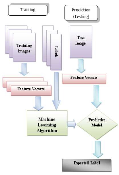
Figure 6. Principal stages of image classification system

• VII.    EXPERIMENTAL SETUP

• A. Blocking of Image

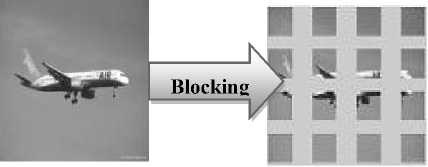
Blocking model is the concept of dividing the given image into equal sub-block images. The size of the sub-block depends on the size of the original image. In this work image of size 128x128 pixels is divided into four sub-blocks of size 32x32 horizontally and four sub-blocks of size 32x32 vertically, i.e. each original image is divided in 16 blocks as shown in fig 7. Six features mentioned in section 2 from each sub image are calculated. This gives a feature vector of size 96 for each image. This procedure of feature extraction is applied in all three experiments as follows

Original Image of size 128x128

Blocking

Figure 7. Blocking of Image into 32x32 blocks

B. Experiment 1

The first experiment is carried out on data set containing 16 classes and 50 images of each class for

training and 100 images of each class for testing. Initially the original images are resized to 128X128 pixels and then features are extracted using blocking model as described above. It produces a feature matrix of size 96X800. Similarly 96X1600 feature matrixes are produced for testing images. Then a neural classifier is designed with fifteen hidden layers and 16 output layers. Feature matrix of training images are used to train the neural network. After that they are tested on feature matrix of test image. Then performance of the system is measured

• C.    Experiment 2

Second experiment is performed on noisy data set of 16 classes with 50 images each class for training of feed forward neural network and 100 images each class for testing. This gives poor classification accuracy.

• D.    Experiment 3

Classification of noisy images starts with detection of noise type followed by appropriate filtering operation. This experiment is performed on noisy data set after filter operation on 16 classes with 50 images of each class for training and 100 images of each class for testing Then similar approaches are followed for feature extraction as discussed in above experiments. This gives a good classification accuracy.

• E.    Design of Neural Network

After extraction of features from training and test samples feed forward neural network is designed with the following parameters

No. of hidden layers: 15

No. of output layers: 16

Training Algorithm: Levenberg-Marquardt

VIII.RESULTS DISCUSSION

• A.    Image Data Base

  To have a performance analysis the data base is taken from Columbia Object Image Library (COIL-100) [20]. Columbia Object Image Library (COIL-100) is a database of colour images of 100 objects. The objects were placed on a motorized turntable against a black background. Eight hundred images are used for training the neural network, and 1152 are taken for testing.

• B.    Results & Performance

This section describes the performance analysis of proposed multi class image classification. Confusion matrix is one method for performance evaluation of classifier. The following terms are calculated from the output of the simulation

True Positive Rate

True Positives

All Output Positives

True Negatives

True Negative Rate =

All Output Negatives

False Negatives

False Negative Rate =

All Output Negatives

False Positives

False positive Rate =

All Output Positives

TABLE IPERFORMANCE COMPARISON

Image Class	Experiment 1	Experiment 2	Experiment 3
1	86.8	38.6	59.9
2	90	26.5	66.5
3	90	36.5	62.3
4	77.2	45.8	61.9
5	78.2	38.9	70.5
6	76.8	34.5	69.6
7	83.2	39.5	63.2
8	78.65	31.9	66.4
9	86.4	32.5	38.6
10	86.9	40.5	56.4
11	88.1	38.9	52.9
12	82.6	35.8	37.5
13	84.8	24.9	68.5
14	88.3	39.5	76.5
15	90.2	49.5	82.6
16	80.85	42.8	87.8
Average Classificat ion	84.31	37.28	63.81

• C.    Performance Comparison under different constraints

This work deals with classification of multi class images under different constraints of data set. The first experiment is carried out on images without noise, second with Gaussian noise and filtered data set in third experiment. Performance of the classifier using statistical texture features is presented in the table 1. It is observed that performance of the first experiment is the best in first data set i.e. data set without noise in both the approach, while the performance is decreased if the same images are affected by Gaussian noise as shown in performance graph of fig 8. This is because the texture feature of the original images consists Gaussian noise pattern also. Filtering of the noise from the second data set improves the result. The table also shows that feature extraction using blocking of the image enhance the average classification rate in all the case.

• IX. CONCLUSION

In this paper we have presented a novel approach to perform classification in large category of datasets with different spatial conditions. We demonstrate the technique over the problem of object recognition and classification in noisy image data sets. The results show very little loss of performance for large gains in terms of classification accuracy. In future work, we shall apply the framework with more strong feature set on a much larger dataset, possibly for the task of multi class image classification.

ACKNOWLEDGEMENT

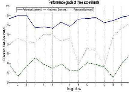
Figure 8. Performance graph of each class