Enhancing the Quality of Medical Images Containing Blur Combined with Noise Pair

Published Online October 2015 in MECS

In medical imaging diagnosis, doctors must rely on the captured images such as computed tomography (CT), magnetic resonance imaging (MRI), etc. to diagnose abnormal defects or diseases that cause damage to the patient's body, such as bone fractures, brain tumors, etc. The diagnosis depends on the skills of the doctors and image clarity. The quality of medical images depends on the environment, capture device, person’s shooting skills, etc. In the real world, most of medical images contain of noise and blur. This problem reduces the quality of images and causes difficulties for viewers (doctors). Medical image noising, blur, noise or pair can have influence on the diagnostic process. A small detail in a medical image is very useful for treatment process. Therefore, denoising and deblurring become popular in image processing. The goal of denoising and debluring is to remove noise and blur details from the corrupted image while maintaining edge features.

In the past, many methods have been proposed for denoising and deblurring such as wavelet transform [1, 2, 3], contourlet transform [5], nonsubsampled contourlet transform [6,  7], ridgelet transform [8], curvelet transform [9, 10, 11], etc. Most of these methods use thresholdings for the process of improvement. Many thresholdings are proposed such as [4, 23, 24]: stationary, cycle-spinning, steerable wavelet transforms, etc. The results were significantly improved when the above methods were used. However, the cases of image denoising or deblurring are very hard work and still a great challenge. Especially, with the pair case, which has blur combined with noise, it is more difficult.

The curvelet transform [11], a new X-let transform multiscale transform, is like the wavelet transform but it has the directional parameters, which contains elements with a very high degree of directional specificity. The results of curvelet transform for denoising are good in some other cases. However, it still needs to continue to be improved. Augmented lagrangian method [13] has given the good results, especially for deblurring or denoising, but the results are not good in case of blur and noise pair. In paper [12], the authors proposed a new method for denoising images, which is based on multilevel threshold in curvelet domain combined with cycle spinning for good results. Mingwei [16] proposed the applying bayesian thresholding in nonsubsampled contourlet transform. With these ideas, we think that the combined methods and thresholdings can give the good result to each process. The initial results are given our previous algorithms in [25, 26] which presented the combination between transform and thresholding. In this paper, we have proposed a method for increasing the quality of medical images in case that blur combined with noise pair is available in medical images. The proposed method is divided into two steps: denoising and deblurring. We use curvelet transform combined with bayesian thresholding for the denoising step and use augmented lagrangian method for the deblurring step. For demonstrating the superiority of the proposed method, we have compared the results with the other recent methods available in literature such as: discrete wavelet transform (DWT) [2], curvelet transform [11] and augmented lagrangian [13]. For performance measure, we have used Peak Signal to Noise Ratio (PSNR) and Mean Square Error (MSE) and it has shown that the results of the present method are better than the other methods. The rest of the paper is organized as follows: in section II, we describe the basic of curvelet transform, principle bayesian thresholding and augmented lagrangian method, which we used; details of the proposed method are given in section III; the results of the proposed method are presented in section IV and our conclusions are made in section V.

• II.    Background

• A.    Curvelet Transforms

Ridgelet transforms [8] in two dimensions provide a sparse representation of smooth functions and perfectly straight edges. Rigelet transforms occur at all scales, locations and orientations; and each has global length and variable widths. And ridgelets have two approaches: monoscale and multiscale ridgelets. Ridgelets combined with a spatial bandpass filtering operation to isolate different scales were curvelets.

Curvelets [11] are better than wavelet based transforms in case of representing edges and other singularities along curves. Curvelets can be translated and dilated, similar to wavelet transforms. On the first decomposing an image into subbands, the curve of curvelets is displayed with width ~ length². After decomposing, each scale is analyzed by a local ridgelet transform. Similar to ridgelets at occuration; but, while ridgelets have global length and variable widths, curvelets in addition to a variable width have a variable length and so a variable anisotropy.

The basic process of the digital realization for curvelet transforms can be summarized [11, 12]:

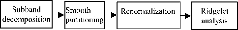
Fig. 1. The process of curvelet transforms.

f irstly , Subband decomposition. The image f is decomposed into subbands:

f h^( P o f , A i f , A 2 f ,...)           (1)

Secondly , Smooth partitioning. Each subband is smoothly windowed into “squares” of an appropriate scale (of sidelength ~2^-s):

A s f l->( W_Q A s f ) q^          (2)

where w is a collection of smooth window localized around dyadic squares:

Q = [ k / 2 ^s ,( k + 1) / 2 ^s ] x [ k ₂ / 2 ^s ,( k ₂ + 1) / 2 ^s ]

Thirdly , Renormalization. Each resulting square is renormalized to unit scale:

g Q = ( T q ) ^{- 1}( W q a s f ), Q e Q s        (4)

Finally , Ridgelet analysis. Each square is analyzed via the discrete ridgelet transform.

In this definition, the two dyadic subbands [22s, 22s+1] and [22s+1, 22s+2] are merged before applying the ridgelet transform.

• B.    Bayesian Thresholdings

Most of the existing thresholding procedures are essentially minimax. They do not take into account some specific properties of a concrete object in which we are interested. Now, we specify a prior distribution on the wavelet coefficients within a bayesian framework.

The estimate noise variance σ and signal variance δ can be obtained by equation [14]:

σ=

^ median (| w i,j| ) ) 0.6745

and

δ2 =max

MN

1         w2 -σ2,0

MxN t=1 j=1 ^t,j

where w i, j is the lowest frequency coefficient after the transformation, MxN is the sub-band’s size.

Abramovich [14] proposed a Bayesian formalism which gives rise to a type of wavelet threshold estimation in nonparametric regression. They establish a relationship between the hyperparameters of the prior model and the parameters of those Besov spaces within which realizations from the prior will fall. The bayesian threshold solves the standard nonparametric regression problem [14]:

y. = g(t i ) +e , ., i = 1,..., n           (7)

where h=i/n and G. are independent identically distributed normal variables with zero mean and variance 5 ², and they will recover the unknown function g from the noised data without assuming any particular parametric form.

Bayesian thresholdings based on discrete wavelet transforms. The discrete wavelet coefficients are defined by the vector of function values. Based on this vector, which rules, apply them to hard and soft thresholding. In the hard thresholding, the important coefficients remain unchanged while the important coefficients are reduced by the absolute threshold value in the soft thresholding.

• C.    Augmented Lagrangian Method

A linear shift invariant imaging system is modeled as [13]:

g = Hf + η                  (8)

where f e R MN ^X1 is a vector denoting the unknown (potentially sharp) image of size M x N, g e R MN ^X1 is a vector denoting the observed image, n e R MN ^X1 is a vector denoting the noise, and the matrix H e R MN ^{X MN} is a linear transformation representing convolution operation. And the goal of image restoration is from the observed image g , algorithms will recover f .

The algorithm is proposed to minimize a total variation optimization problem for spatial-temporal data by Stanley [13]. This algorithm uses an augmented lagrangian method to solve the constrained problem. Two problems are considered as TV/L1 and TV/L2 minimization are defined as:

minimize   ^|\Hf - g ||² +|| ^f||₇._r            ⁽⁹⁾

and minimize д|Hf - g||1 +| f/;         (10)

With equations, μ is the regularization parameter. The idea of the augmented lagrangian method is to find a saddle point. And we can use the alternating direction method (ADM).

The idea of augmented lagrangian is to find a saddle point of L(f, u, y); then, they use the alternating direction method (ADM) to solve f-subproblem, u-subproblem with TV/L2 and f-subproblem, u-subproblem and r-subproblem with TV/L1. The equation as [13]:

minimize ^μ Hf-g ² + u           (11)

and minimize ^||r || ₁+||u||₁            (12)

Subject to r = Hf - g and u = Df. Algorithm of TV/L1 or TV/L2 can be summarized as follows [13]:

• (i)    Input: vector denoting the observed image and convolution matrix, regularization parameter, the isotropic total variation.

• (ii)    Set parameter with value default for each types of TV/L1 or TV/L2.

• (iii)    Initialize for the first value, such as: f, u.

• (iv)    Compute the matrices of the first-order forward finite difference operators along the horizontal, vertical and temporal directions.

• (v)    With not coverage do:

+ Solve the sub problems and update parameter.

+ Check convergence, if false continue.

• III.    The Proposed Method for Image Denoising Combined with Deblurring

Blur images are very difficult for image processing, especially with images which consist of blur and noise pair. In this section, we propose a new approach for image deblurring, with blur and noise pair based on curvelet transforms combined with bayesian thresholding and augmented lagrangian method.

Curvelets and ridgelets take the form of basic elements, which exhibit very high directional sensitivity and are highly anisotropic. Curvelet transforms, based on the principle of anisotropic scaling, have given entirely different scale an isotropy of wavelet transforms.

As mentioned in section 1, Starck [11] used the curvelet transform for image denoising. Do [6] developed the contourlet transform using a double filter bank structure for denoising. Donoho [5] proposed the ridgelet transform and using it for denoising. The ridgelet transform is not sufficient to handle linear discontinuities in images. Donoho [8] proposed the curvelet transform by utilizing the properties of the ridgelet transform. To compensate for the lack of translation invariance property of the curvelet transform, we apply the principle of bayesian thresholding for image denoising. Because the thresholding may overcome this disadvantage. Bayesian thresholding for deblurring images [15, 22] is based on the median of thresholding and the denoising [15] for noise images are not at all. We proposed the combination in [25] which use ridgelet transform and bayesian thresholding for denoising step, then we apply the Wiener filter for deblurring step in denoising images. With deblurring, augmented lagrangian method [13] is the very excellence method for deblurring process. In [26], we use the curvelet transform for denoising step and augmented lagrangian for deblurring step. But with [26], in many types of noise or blur, we not chance algorithm for each types. Therefore, we divide medical image processing with the blur and noise pair into two processes: denoising and deblurring, and chance the algorithm to depend on each types blur or noise. The proposed method includes two steps. The proposed method is used as figure 2:

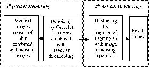
Fig. 2. The processing of proposed method.

Firstly, the inputs are the blur combined with noise in images. We use curvelet transforms for denoising images, the process of curvelets is as follows [11]:

(i) apply the b 1 =b min

à trous algorithm with scales and set

• ( ii) for. j=1, .„, j do

• +    partition the subband w j with a block size b j and apply the digital ridgelet transform to each block;

• +    if j modulo 2 = 1 then b j+1 =2b j  else b j+1 =b j

The sidelength of the localizing windows is doubled at every other dyadic subband.

Bayesian thresholding is the composition in wavelet transforms, calculates median thresholding and shows result based on the new thresholding. The process of bayesian thresholding can be achieved as follows:

After this period, the input images become denoising images. The result of denoising with curvelet transforms combined with bayesian is good in the types of noise, such as: gaussian, speckle, etc.

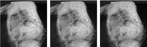
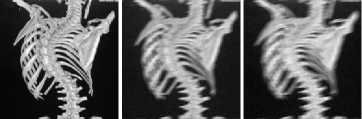
Figure 3 shows the denoising image in case of speckle noise using curvelet transforms combined with bayesian thresholdings.

(d)                         (e)

Fig. 3. A noise image with speckle noise and denoising images by different methods.

• (a)    Original image.

• (b)    Noise image (PSNR = 20.0232 db).

• (c)    Denoising image by DWT (PSNR = 22.7776 db).

• (d)    Denoising image by curvelet transforms (PSNR = 28.8155 db).

• (e)    Denoising image by curvelet transforms combined with bayesian thresholdings (PSNR = 29.0008 db).

From figure 3, the result of the method, curvelet transforms combined with bayesian thresholdings, is the highest. But with Gaussian noise, we use db2 for decomposition and db4 in speckle noise. The results are very satisfactory because Gaussian noise is the summation and speckle noise is the multiplication.

The summation is the noise value will add in each pixel of medical images. So, decomposition needn’t high level. The multiplication is the noise value will accumulate in each pixel of medical images. Removed the multiplication noise must double decomposition value.

Secondly , it is medical image deblurring. The noise in the blur combined with noise images has been removed in the curvelet domain in the above period. The blur in images is not removed more. To remove the blur, we use augmented lagrangian for the output images from the previous period.

In here, we use augmented lagrangian TV/L2 algorithm [13] to remove the blur. The problem that we solve in TV/L2 minimization is:

minimize ^|\Hf - g ||² +|I f^          ⁽¹³⁾

Algorithm of TV/L2, which is used in the proposed method, can be summarized as follows [13]:

• (i)    Input: vector denoting the observed image (g) and convolution matrix (H), regularization parameter Ц , the isotropic total variation Д , в , Д ■

• (ii)    Set parameter with value default for p = 1 ( p is a regularization parameter) for Gaussian blur and p = 2 for motion blur. Then set a = 0.7.

The reason of this choice: Gaussian blur is to strengthen the standard deviation, but motion blur is the movement of objects and sightseeing. Therefore, we set default for regularization parameter of Gaussian blur is 1 and motion blur is 2.

• (iii)    Initialize f 0 = g, u 0 = Df 0 , y = 0, k = 0. (y is the Lagrange multiplier)

• (iv)    Compute the matrices of the first-order forward finite difference operators along the horizontal, vertical and temporal directions.

With not coverage do:

• 1.    Solve the f-subproblem is:

f t _{+ 1} = arg min ^ | H - g ||² - y t ⁽ u_t - D ^f ) + ^p u u_t - D ^f ||² f 2                             2

by equation:

F [ _M H^Tg + p , Du - Dy ]

_A| ^F [ H ] ² + p , ( ^F [ D , ] ² + F [ ^D y Л ² + F [ ^D t ] ² )

where F denotes the three-dimensional Fourier Transform operator.

2. Solve the u-subproblem is:

PSNR=20log (

MAX

MSE

)

u k + 1= argmini | u | L - y T ⁽ u - Df k ₊i ) + ^-Wu - Df k ₊i||2 u 2

by equation:

ux = max ] Ivxl- — ,0f * sign (vx )

I      PrJ

3. Update the Lagrange multiplier:

Ук+1 = yk - Pr(uk+1 - Dfk+1)

where MAX 1 is the maximum pixel value of the image. The proposed method is compared with DWT, CT, and AL method based on the MSE and PSNR values. The smaller the value of MSE is, the better it is. The higher the value of PSNR is, the better it is. We test so many medical images. In here, we show some test cases.

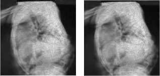
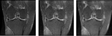
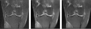
Figure 4 shows the deblurring of blur and noise image which has Gaussian blur combined with Gaussian noise by our proposed method. Figure 5 shows the deblurring of blur and noise image which has Gaussian blur combined with Speckle noise by our proposed method.

4. Update:

(a)                 (b)                 (c)

P r

={

YP r ^{, if} || u k +1 ^- Df k +11₂ ^ 4 u k ^- Df k 11₂ p _r , otherwise

5. Check convergence: if

(d)                   (e)                   (f)

Fig. 4. Denoising and deblurring images in case Gaussian blur is combined with Gaussian noise by different methods.

II f + 1 - f k lLI f lL s tol         (20)

then break, else continue.

IV. Experiments and Results

In this section, we apply the procedure described in section 3 and achieved superior performance in our deblurring experiments as demonstrated in this section. For performance evaluation, we compare the results of the proposed method based on curvelet transforms combined with bayesian thresholdings and augmented lagrangian (CTBTAL) with the methods: discrete wavelet transform (DWT), curvelet transforms (CT) and augmented lagrangian (AL). We test the result in medical image datasets, this dataset includes different images of different sizes: 256x256, 512x512. Hard thresholding is applied to the coefficients after decomposition in the curvelet domain. All of the above methods are done on our program and the same images at the similar scale.

The quality of images is improved by comparison with the value of Mean Square Error (MSE) and Peak Signal-to-Noise Ratio (PSNR). The MSE is defined as:

• (a)    Original image.

• (b)    Blur combined with noise in image (PSNR = 25.2391db).

• (c)    Denoised and deblurred image by DWT (PSNR = 28.0690 db).

• (d)    Denoised and deblurred image by AL (PSNR = 26.0581db).

• (e)    Denoised and deblurred image by CT (PSNR = 27.8005db).

• (f)    Denoised and deblurred image by CTBTAL (PSNR = 29.0626 db).

(d)                  (e)                   (f)

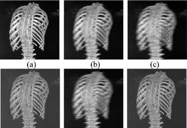
Fig. 5. Denoising and deblurring images in case Gaussian blur is combined with Speckle noise by different methods.

NN

MSE= ¹       (x -y ) ²

NxN i=1 j=1 ^{i,j i,j}

where x is the image which has blur and noise, y is the image result and N x N is the size of image. PSNR is used as the measure of quality of reconstruction of image deblurring or denoising, defined as:

• (a)    Original image.

• (b)    Blur combined with noise image (PSNR = 28.9375 db).

• (c)    Denoised and deblurred image by DWT (PSNR = 29.4235 db).

• (d)    Denoised and deblurred image by AL (PSNR = 30.5175 db).

• (e)    Denoised and deblurred image by CT (PSNR = 29.8517 db).

• (f)    Denoised and deblurred image by CTBTAL (PSNR = 31.5662 db).

From figure 4 and figure 5, we see that the result of the proposed method (fig.(f)) is better than the other methods (fig.(c), fig.(d), fig.(e)). Figure 6 show the plot

of PSNR, MSE values of different image deblurring and denoising methods corrupted in case of Gaussian blur combined with Gaussian noise.

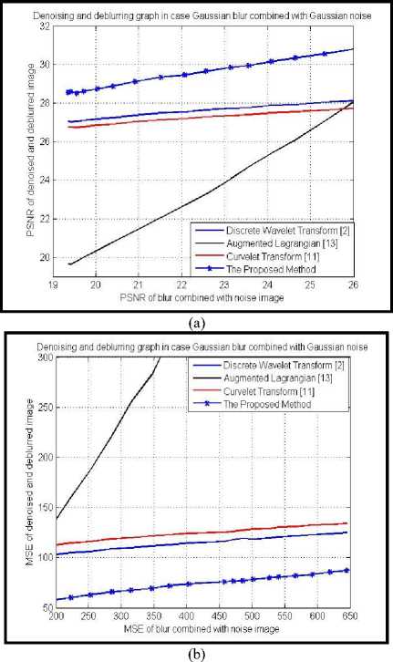
Fig. 6. Plot of PSNR and MSE values of denoised and deblurred images in case of Gaussian blur combined with Gaussian noise using different methods.

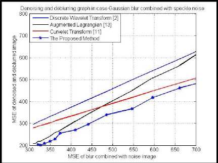
(b)

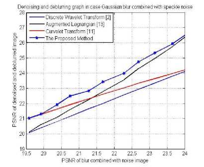
Fig. 7. Plot of PSNR and MSE values of denoised and deblurred images in case of Gaussian blur combined with speckle noise using different methods.

• (a)    Plot of PSNRvalues of denoised and deblurred images.

• (b)    Plot of MSE values of denoised and deblurred images.

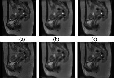
Figure 8 shows the deblurring of blur and noise image in case of motion blur combined with Gaussian noise by our proposed method and the other method. Figure 9 also shows the deblurring of blur and noise image in case of motion blur combined with speckle noise by our proposed method and the other method.

(a)

c)

• (a)    Plot of PSNRvalues of denoised and deblurred images.

• (b)    Plot of MSE values of denoised and deblurred images.

  Figure 7 show the plot of PSNR, MSE values of different image denoising and deblurring methods corrupted in case Gaussian blur combined with speckle noise.

  

  (a)

  
  

(d)                   (e)                  (f)

Fig. 8. Denoising and deblurring images with motion blur combined with Gaussian noise by different methods.

• (a)    Original image.

• (b)    Blur combined with noise in image (PSNR = 16.9468 db).

• (c)    Denoised and deblurred image by DWT (PSNR = 17.5966 db).

• (d)    Denoised and deblurred image by AL (PSNR = 20.0532 db).

• (e)    Denoised and deblurred image by CT (PSNR = 17.6140 db).

• (f)    Denoised and deblurred image by CTBTAL (PSNR = 22.6687db).

  

  (d)                   (e)                  (f)

  Fig. 9. Denoising and deblurring images in case of motion blur combined with speckle noise different methods.

  
  

  • (a)    Original image.

  • (b)    Blur combined noise image (PSNR = 17.2759 db).

  • (c)    Denoised and deblurred image by DWT (PSNR = 17.4074 db).

  • (d)    Denoised and deblurred image by AL (PSNR = 20.1790 db).

  • (e)    Denoised and deblurred image by CT (PSNR = 17.6344 db).

  • (f)    Denoised and deblurred image by CTBTAL (PSNR = 20.9319 db).

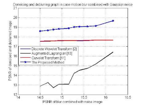
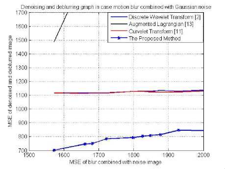
From figure 8 and figure 9, we see that the result of the proposed method fig.(f) is better than the other methods (fig.(c), fig.(d) and fig.(e)). Figure 10 show the plot of PSNR, MSE values of different image denoising and deblurring methods corrupted in case of motion blur combined with Gaussian noise.

(a)

(b)

Fig. 10. Plot of PSNR and MSE values of denoised and deblurred images in case of motion blur combined with Gaussian noise using different methods.

• (a)    Plot of PSNRvalues of denoised and deblurred images.

• (b)    Plot of MSE values of denoised and deblurred images.

Figure 11 show the plot of PSNR and MSE values of different image denoising and deblurring methods corrupted in case of motion blur combined with speckle noise.

With figure 6, figure 7, figure 10 and figure 11, the PSNR values of the proposed method is the highest and the MSE values of the proposed method is the smallest. So, the proposed method performs better than discrete wavelet transform, curvelet transform and augmented lagrangian method. As mentioned in section 3, we improve the denoising processing. Therefore, the proposed method is better than the other method.

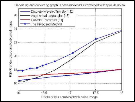
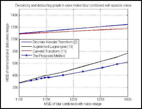
Fig. 11. Plot of PSNR and MSE values of denoised and deblurred images in case of motion blur combined with speckle noise using different methods.

• (a)    Plot of PSNRvalues of denoised and deblurred images.

• (b)    Plot of MSE values of denoised and deblurred images.

• V. Conclusions

In this paper, we proposed the method for increasing the quality of blur combined with noise image by dividing it into two processes: denoising and deblurring. Firstly, we propose a new method for denoising image based on curvelet transform combined with bayesian thresholding. Then, we apply augmented lagrangian method for deblurring into denoising image. We test the proposed method with Gaussian blur combined with Gaussian noise pair, Gaussian blur combined with speckle noise pair, motion blur combined with Gaussian noise pair, and motion blur combined with speckle noise pair in medical images. From the results of the above section, we conclude that the proposed method works well and better than the other recent methods available in literature such as: discrete wavelet transforms, curvelet transforms and augmented lagrangian. Based on this idea, we think the combination methods can improve the quality of the image which has blurring and noising in case of denoising and deblurring step. Furthermore, we can develop this idea by combining thresholdings or filters in the deblurring or denoising step.

Appendix

Table 1. PSNR values (dB) of different denoised and deblured images with Gaussian blur combined with Gaussian noise.

Test Image	Image Size	Blur & Noise Image	DWT[2]	AL [13]	CT[11]	Proposed Method
1	256 x 256	21.3958	25.3283	22.0264	25.1122	26.0232
2		20.6148	23.7412	21.0870	23.8914	24.7274
3		21.8062	25.0981	22.5222	25.2357	26.3515
4		19.3783	23.5501	19.6916	23.6754	24.9114
5		17.8001	24.9717	17.7717	24.9701	25.4818
6		16.0633	20.5249	16.3098	20.3469	21.1879
7		15.6079	22.3795	15.5836	22.2922	22.9893
8		14.9423	22.3773	14.8368	22.4524	23.1188
9		26.6524	31.6191	27.6351	31.3123	33.4234
10		24.1366	27.6435	25.0279	27.4658	29.4094
11	512 x 512	24.8521	32.9369	25.3458	32.5904	33.8393
12		21.7640	24.9861	22.7562	24.6530	26.2621
13		20.9965	23.5191	22.2377	23.1775	25.1051
14		24.2241	31.0421	24.8162	30.5948	32.3928
15		26.0221	31.8145	26.8493	31.3897	33.2971
16		20.0243	23.8463	20.8065	23.4914	25.4073
17		19.7131	23.8335	20.4062	23.4848	25.0111
18		21.2679	27.3645	21.8067	27.0792	29.2639
19		22.3948	28.6748	22.8228	28.3454	29.5994
20		23.9863	30.3258	24.5808	30.0443	31.6380

Table 2. PSNR values (dB) of different denoised and deblured images with Gaussian blur combined with speckle noise.

Test Image	Image Size	Blur & Noise Image	DWT[2]	AL[13]	CT [11]	Proposed Method
1	256 x 256	23.0920	25.5998	24.1175	25.3611	26.4193
2		20.2344	20.5992	20.5848	22.9130	23.2919
3		21.6390	21.7473	21.8942	21.7346	22.6895
4		17.5646	18.1684	17.5961	20.6789	20.9086
5		17.4910	21.0917	17.3516	24.2070	24.2351
6		18.1855	19.419	18.7048	20.5158	21.2482
7		22.4617	23.0035	23.6952	24.4640	25.9205
8		23.2818	23.9857	24.8751	25.1727	27.0829
9		23.8397	23.9484	23.9366	23.9670	24.1572
10		25.3260	25.7947	26.7436	27.2852	28.7624
11	512 x 512	25.9560	26.7559	26.1194	28.1989	28.2931
12		21.6175	23.8826	22.4633	24.5813	25.7629
13		21.0589	21.3584	22.2705	21.8535	22.8422
14		26.8943	27.4241	27.3779	28.2239	28.6356
15		22.6899	23.4968	22.8497	25.0090	25.4673
16		24.1621	24.2359	26.9951	24.2192	27.0083
17		20.7494	21.1499	21.5973	21.9186	22.4882
18		22.4913	23.2765	22.9129	24.0157	24.0499
19		24.6980	25.1384	25.2960	26.0356	26.0793
20		21.4004	21.7755	22.4325	22.3737	22.9852

Table 3. PSNR values (dB) of different denoised and deblured images with Motion blur combined with Gaussian noise.

Test Image	Image Size	Blur & Noise Image	DWT[2]	AL[13]	CT [11]	Proposed Method
1	256 x 256	23.0159	23.9126	24.1707	23.9211	25.4899
2		20.4164	21.5119	20.7121	21.6111	23.3620
3		18.7250	19.9783	19.4557	20.0889	22.9818
4		18.1161	20.0751	17.6501	20.1666	22.6791
5		19.6700	23.3954	17.5249	23.3652	24.3956
6		16.1661	17.6504	16.4068	17.6499	19.6690
7		16.3928	18.1925	15.8901	18.1829	20.7334
8		15.6207	18.6812	13.6431	18.6463	20.4013
9		17.6315	23.0562	14.6550	23.3315	23.8703
10		14.9204	20.6489	11.6314	20.8879	21.0647
11	512 x 512	15.0977	24.8670	11.4825	24.5610	24.8837
12		11.7964	19.4221	8.3987	19.3432	19.8086
13		11.3582	16.6619	8.4165	16.7060	17.1649
14		16.2420	22.8994	13.1730	23.1072	23.9144
15		14.6604	23.3671	11.0207	23.3920	23.6629
16		14.7424	17.6907	13.4450	17.6841	20.1851
17		13.4890	17.5244	11.2170	17.6103	19.0756
18		17.1167	21.5949	14.8758	21.6374	23.8379
19		17.1765	22.4123	14.5668	22.5664	23.7518
20		14.9819	22.5403	11.6565	23.0844	23.2075

Table 4. PSNR values (dB) of different denoised and deblured images with motion blur combined with speckle noise.

Test Image	Image Size	Blur & Noise Image	DWT[2]	AL[13]	CT [11]	Proposed Method
1	256 x 256	22.4100	24.7134	21.2940	24.6266	25.5927
2		19.1920	19.5068	17.5274	21.1395	21.3500
3		20.4008	20.3845	20.8618	20.4732	21.0328
4		17.7349	18.1884	15.5692	18.6866	20.0897
5		18.4259	21.3622	15.1831	22.6422	23.9545
6		18.5827	18.8027	20.9717	18.9451	21.5676
7		17.3083	18.0587	16.5054	19.5437	19.5775
8		16.8926	18.2756	14.1685	20.3064	21.0873
9		22.4852	22.8350	22.2780	23.9468	25.0694
10		19.7566	20.5159	17.2242	21.3251	22.9169
11	512 x 512	22.8737	23.4814	21.2150	23.2188	24.5355
12		18.1377	19.4882	18.1496	19.8776	22.0791
13		16.2261	16.4821	16.6008	16.9632	17.8333
14		19.8124	20.3238	17.8346	18.9662	21.2454
15		20.9099	21.5762	18.8455	21.0078	22.8969
16		16.0032	16.3796	16.2427	16.9603	17.8581
17		15.9016	16.2572	15.5399	16.9014	16.9627
18		18.0265	18.7282	16.0603	17.1930	19.4643
19		18.1800	18.7034	15.7661	17.3751	19.8848
20		19.8650	20.2711	18.5455	19.8791	21.0384

Acknowledgment