Ergodic Capacity of MIMO Channel in Multipath Fading Environment

Published Online September 2013 in MECS

Wireless systems continue to strive for ever higher data rates. This goal is particularly very challenging as most of the systems are power, bandwidth, and complexity limited. However, using the multiple transmitter and receiver the channel capacity can be significantly increased. Foschini [1] and Telatar [2] ignited much interest in this area by predicting remarkable spectral efficiencies for wireless systems with multiple antennas when the channel exhibits rich scattering and its variations can be accurately tracked.

The large spectral efficiencies associated with MIMO channels are due to the fact that a rich scattering environment provides independent transmission paths from each transmit antenna to each receive antenna.

Therefore, for single-user systems achieves a capacity min(N ,N )

on approximately         ^TR separate channels,

NN where T is the number of transmit antennas and   R is the number of receive antennas. Thus, it can be stated that the capacity scales linearly with min(NT, NR)

relative to a system with just one trans mit and one receive antenna. This capacity increase requires a scattering environment such that the matrix of channel gains between transmit and receive antenna pairs has full rank and independent entries, and that perfect estimates of these gains are available at the receiver. Still the question remains open that the enormous capacity gains initially predicted [1-2] can be obtained in more realistic operating scenario, and what are the specific gains that results from adding more antennas and/or a feedback link between the receiver and transmitter.

We focus on MIMO channel capacity in the Shannon theoretic sense. The Shannon capacity i.e., the maximum mutual information of a single-user time-invariant channel corresponds to the maximum data rate that can be transmitted over the channel with arbitrarily small error probability.

When the channel is time varying, the channel capacity has multiple definitions, depending on what is known about the instantaneous channel state information (CSI) at the transmitter and/or receiver and whether or not capacity is measured based on averaging the rate over all channel states or maintaining a fixed rate for most channel states. More particularly, when CSI is known perfectly both at transmitter and receiver, the transmitter can adapt its transmission strategy relative to the channel and therefore channel capacity is characterized by the ergodic, outage, or minimum rate capacity. Ergodic capacity can be defined as: the maximum average rate under an adaptive transmission strategy averaged over all channel states (long-term average). The Outage capacity define as: the maximum rate that can be maintained in all channel states with some probability of outage (no data transmission).

The Minimum rate capacity define the maximum average rate under an adaptive transmission strategy, that maintains a given minimum rate in every channel state, and then averages the total rate in excess of this minimum over all channel states. When only the receiver has perfect knowledge of the CSI then the transmitter must maintain afixed -rate transmission strategy based on knowledge of the channel statistics only, which can include the full channel distribution, just its mean and variance (equivalent to the full distribution for complex Gaussian channel gains), or just its mean or variance. In this case Ergodic capacity define, the rate that can be achieved via thisfixed -rate strategy based on receiver averaging over all channel states [2-6]. Alternatively, the transmitter can send at a rate that cannot be supported by all channel states, in these poor channel states the receiver declares an outage and the transmitted data is lost. In this scenario each transmission rate has an outage probability associated with it and capacity is measured relative to outage probability (capacity CDF) [1].

In this paper, MIMO system model is discussed in section II. The capacity of the MIMO channels under different condition is discussed in section III. In section IV, the channel capacity is estimated for SISO, SIMO, MISO and MIMO channels. The channel capacity for the random MIMO channels is also estimated through simulation in section V. MIMO Channel Capacity in the Presence of Antenna Correlation Effect is detailed in section VI. Finally, the major conclusion of the paper is discussed in section VII of the paper.

• II.    MIMO System Model

Consider a transmitter with N transmits antennas, and a receiver with M receives antennas. The channel can be modeled by the N ^x M matrix H , where H is Channel Matrix The N ^{x 1} received signal y is [5].

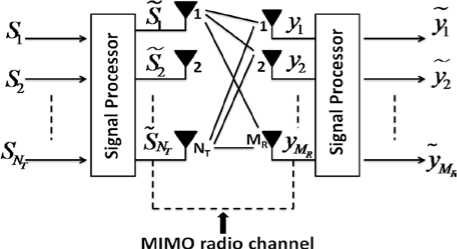
Fig. 1: MIMO system model.

y = Hs + n .

s

Where s is the transmitted symbol (s1, s2, s3,……, ^NT ) and the covariance matrix for this transmitted signal is given by:

E

R =---I., where, E / N„ is equal to the power of ss NNT      sT each antenna. In the formula (1), the H can be defined as:

Table 1: List of Symbols

Symbol	Parameter/abbreviation
N T	Transmit antennas
N R	Receive antennas
H	Channel matrix
S	Transmitted symbol
n	Noise
Y	MIMO signal
C	Channel capacity
N 0	Identical noise power
E S	Total transmitted Power
SNR	Signal to Noise Ratio
HH	Hermitian matrix
IN	Identity matrix
X	Positive Eigen values of HHH
G	Gain
r	Rank of matrix
R	Correlation Matrix
N 0 /2	Noise PSD (Power Spectral Density)
£	Outage capacity
C OL	Channel Capacity for the Open-Loop
C CL	Channel Capacity for the Closed-Loop
SISO	Single Input Single Output
SIMO	Single Input Multiple Output
MISO	Multiple Input Single Output
MIMO	Multiple Input Single Output

h11   h12 ........ h1M h21 h22 ........ h2M

.             .           .........

h N 1 h N 2........ h NM

Where hij is a Complex Gaussian random variable that models fading gain between the jth transmit antenna and ith receive antenna.

• III.    Capacity of MIMO System:

In the estimation of the capacity of a MIMO system which consists of N transmitting and M receiving antennas, the transfer matrix (H) of the system must be determined. However, there is one more important parameter is channel state information (CSI), and this CSI may be known/ not known at the transmitter/receiver. When the channel state information is not known at the transmitter the capacity is given by [4]

C = log 2

SNR det I IN +     HHH

I n

Where det{.} and {.}H denote the determinate and the

Hermitian (complex conjugate transpose) of a matrix respectively, SNR is the total average Signal to Noise Ratio equally distributed to each transmit antenna element and IN is the ^{N x N} identity matrix.

• 3.1    CSI is known/not known at the transmitter

  • 3.1.1    Channel Capacity when CSI is available at the Transmitter

In this case, the channel capacity is given as [4]

C = log 2 d^et I^

E      ^

+-- s— HH H

N t N o     J

Using the eigen-decomposition

HH H = Q Л Q ^H and the identity where A G C m ^x ” and B G C ” ^{x m} , the channel capacity in (5) is expressed as:

When the channel state information available at the transmitter, modal decomposition can be performed as shown in the figure 2, in which a transmitted signal is prior with V in the transmitter and then, a received signal is post processed with UH in the receiver [3].

C = log₂ det

Г

I_N +        HH ' = log₂det

I N R N t N o     J

Г F

In + —— Л

I N R N t N o

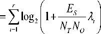
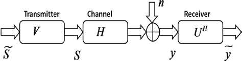
Fig. 2: System model when channel knowledge is availed at the transmitter side.

where r denotes the rank of H, that is, r = Nmin = m i”(NT , Nr ) . From (6), a MIMO channel can be converted into r virtual SISO channels with the transmit power ES/ NT for each channel and the channel gain of Xi for the i th SISO channel. It is

Under this condition the capacity is given by observable that the   (6) is a special case with yi = 1, i = 1,2,....., r, when CSI is not available at

r

C = max ^ log 2

i = 1

^NT^NO ⁱ

r

Subjected to ^ y . = N T .

i = 1

the transmitter and thus, the total power is equally allocated to all transmit antennas.

Considering the case, when the total channel gain is fixed,

for example, H

F

r

= ^ Xi = g, H has i=1

a full rank,

However, the capacity can be increased by resorting to the so called ‘water filling principle’, by assigning various levels of transmitted power to various transmitting antennas. This power is assigned on the basis of the channel performance, that the better the channel gets, the more power it gets and vice versa. This is an optimal energy allocation algorithm.

N T = N_R = N , and r=N , then the channel capacity (6) is maximized when the singular values of H are the same for all the (SISO) parallel channels, that is,

X = — , i = 1,2,..., N .                          (7)

^{i N}

Formula (7) implies that the MIMO capacity is maximized when the channel is orthogonal, i.e,

3.1.2. Channel Capacity when CSI is not available at the Transmitter Side

When H is not known at the transmitter side, one can spread the energy equally among all the transmit antennas, that is, the autocorrelation function of transmit signal vector s is given as.

HH H = H H H = ^— I_N

NN

which leads its capacity to N times that of each parallel channel, i.e.,

Rss = I_Nr

C = N log₂

1 +

— ^E S

N o N J

• IV.    Channel Capacity of SIMO and MISO Channels

In this section the channel capacity is modeled for

SIMO and MISO channel. For the case of a SIMO channel

N with one transmit antenna and R receive antennas, the channel gain is given as h = CNrA and thus r=i and 1 F . Consequently, regardless of the availability of CSI at the transmitter side, the channel capacity is given as

( h^H / h ) s is transmitted instead of s directly.

Therefore, the received signal can be expressed as hH y=T^Sh.   5+z=V^JlIhb+z         (14)

h

Note that the received signal power has been increased

N by T times in formula (14) and thus, the channel capacity is given as

c

SIMO

( E

= ^2 ¹ + _x

V " O

MISO

(            ^        (          ^

= log 2 ¹ + ^^H = log 2 ¹ + ЧТ", V ⁿo 2      V ⁿo 2

If | h | = 1, i = 1,2,...., N _R , and consequently

|h    = N _r , the capacity is given as

C

SIMO

( E, = log 2 1 + -^ N r

V ^N O

A

From (11), it can visualize that the channel capacity increases logarithmically as the number of antennas increases. It is also observable that only a single data stream can be transmitted and that the availability of CSI at the transmitter side does not improve the channel capacity at all.

For the case of a MISO channel, the channel gain is given as, ^{h e C} T , thus r=1 and ^ II^H F when CSI is not available at the transmitter side, the channel capacity is given as

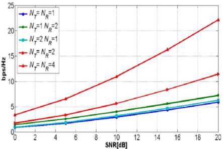
Fig. 3: MIMO channel capacity for SISO, SIMO, MISO, and MIMO when CSI not availed at the transmitter.

MISO = ^log 2 ^{1 +} V

E S N T N O

h ²

A

F

If    h i = 1, i = 1,2,...., N T , and consequently

|h    = NT , the formula (12) reduces to

c

MISO

( f_A

= log 2 1 + - S

V ^N O 2

In figure 3, result are drawn with vary number of transmit and receive for example NT=NR=1 for SISO system, NT=1 and NR=2 for SIMO system and NT=NR=4 is a MIMO system. It is clear from the figure, that the SIMO and MISO channel has nearly same performance. Hence, it can be deduced that, in case of either, single transmitter and signal receiver the performance is same, while as the number of transmitter and receiver increases the performance also.

From the above result, it is evident that the capacity is the same as that of a SISO channel. One might ask what the benefit of multiple transmit antennas is when the capacity is the same as that of a single transmit antenna system. Although the maximum achievable transmission speeds of the two systems are the same, there are various ways to utilize the multiple antennas, for example, the space-time coding technique, which improves the transmission reliability.

• 4.1    CSI is availed at the transmitter side .

When CSI is available at the transmitter side (i.e., h is known), the transmit power can be concentrated on a particular mode of the current channel. In other words,

• V.    Channel Capacity of Random MIMO Channels

• 5.1    Outage channel capacity:

Till now we have assumed that MIMO channels are deterministic. In general, MIMO channels are random in nature. Therefore, H is a random matrix, which means that its channel capacity is also randomly time varying. In other words, the MIMO channel capacity can be given by its time average. In practice, random channel is assumed to be an Ergodic process. Hence, the MIMO channel capacity can be modeled as,

Another statistical notion of the channel capacity is the outage channel capacity. Define the outage probability as с = E {C (H)}

P out ( R ) - Pr( C ( H ) <  R )                     (19)

- E <  max Tr ( R ss ) = N T

^log 2 det I^

+— —hR_ssh^h r

SS

^1N T^1NO             /I

This is frequently known as an ergodic channel capacity. For example, the ergodic channel capacity for the open-loop system without using CSI at the transmitter side, from (6), is given as

Similarly, the ergodic channel capacity for the closed-loop (CL) system using CSI at the transmitter side, is given as:

In other words, the system is said to be in outage if the decoding error probability cannot be made arbitrarily small with the transmission rate ofRbps/Hz. Then, the ^s -outage channel capacity is define as the largest possible data rate such that the outage probability in formula (19) is less than ^s . In other words, it is corresponding to C P ( C ( H ) <  C ) - s .

^E such that ^E/ the capacity for the random MIMO channel can be performed the cumulative distribution function (CDF) when CSI is not available at the transmitter side. Figure 5 and 6 shows the CDFs of the random ^{2 x 6} , ^{2 x 4} MIMO channel capacities when SNR is 10dB, in which ^s =0.1-outage capacity is indicated. It is clear for the figure the outage capacity is same for any value of CDF.

C_CL - E <  max

2 r - 1 Yi=NT

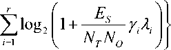
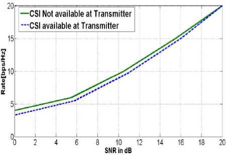
Fig.4: channel capacity comparison when CSI available and not available at the transmitter side for random MIMO channel.

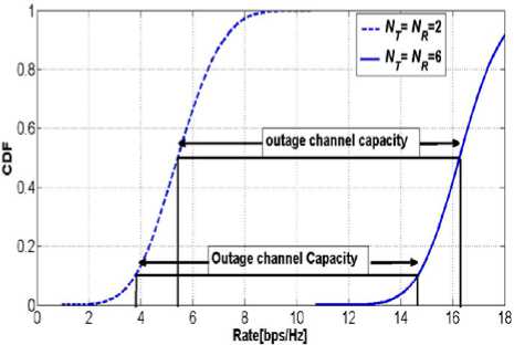
Fig.5: Distribution of MIMO channel capacity (SNR =10dB; CSI is not available at the transmitter side).for N_T=N_R= 2 and N_T=N_R= 6.

In figure 4, data rate Vs SNR is plotted while in presence /absence of CSI at the receiver, it is evident from the figure, that the knowledge of the CSI at the transmitter does not improve the performance of the system. Hence, the knowledge of the CSI at the transmitter is not an important parameter in the designing of the system as far as capacity is concern.

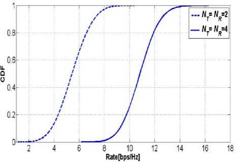
Fig. 6: Distribution of MIMO channel capacity (SNR =10dB; CSI is not available at the transmitter side). for N_T=N_R= 2 and N_T=N_R= 4 .

Comparing the figure 5 and 6 it can be deduced that as the number of NT and NR increases the bit rate as well as the outage capacity increases.

C « log₂ det

E S N T N O

)

H w H Hw + log 2 det( R )

+ ^lo g 2 ^{det( R}t )

VI. MIMO Channel Capacity in the Presence of Antenna Correlation Effect

In general, the MIMO channel gains are not independent and identically distributed. The channel correlation is closely related to the capacity of the MIMO channel. In the sequel, we consider the capacity of the MIMO channel when the channel gains between transmit and received antennas are correlated [6-10]. When the SNR is high, the deterministic channel capacity can be approximated as

From (23) it can be concluded that the MIMO channel capacity has been reduced, and the amount of capacity reduction (in bps) due to the correlation between the transmit and receive antennas is

log₂ det( R r ) + log₂ det( R_t )

In the sequel, it is shown that the value in formula (24) is

C « max , ( R SS ) = N l^ de^{t( R} _ss )

always negative by the fact that og² e ( ) for any correlation matrix R. Since R is a symmetric matrix,

+ log₂ det

E S HH H

^NNO ^ww

eigen-decomposition, that is,

R = Q A Q ^H c

.Since the

determinant of a unitary matrix is unity, the determinant of a correlation matrix can be expressed as

From (20), it is observable that the second term is det( R) = П N, A.

constant; while thefirst term involving

det( R SS )_is

R,, = I., maximized when ^{SS N} . Consider the following correlated channel model:

Note that the geometric mean is bounded by the arithmetic mean, that is,

H = R ^1/2 H w R t ^1/2

( П N = , A i ) N ^ 1 ]E A = ¹

^{1 v} i = 1

R where t is the correlation matrixfl, erceting the correlations between the transmit antennas (i.e., the

R correlations between the column vectors of H),  r is the correlation matrix reflecting the correlations between the receive antennas (i.e., the correlations between the row H vectors of H), and W denotes the i.i.d. Rayleigh fading channel gain matrix. The diagonal entries ofRt and r are constrained to be a unity [11-16]. From (5), then, the MIMO channel is given as

From (25) and (26), it is obvious that log2 det(R) < 0                              (27)

The equality in Formula (27) holds when the correlation matrix is the identity matrix. Therefore, the quantities in (24) are all negative [17-22].

The capacity of the random MIMO channel, while considering the correlation effect is drawn on the figure 7. While considering the channel transfer matrix as shown below:

C = log 2 det( In. + - ^ j- R^1,2 H . R,H;.R r /2 )

N T N O

N = N = NR R

If ^TR , ^r and ^t are of full rank, and SNR is high, Formula (22) can be approximated as

0.76 exp⁰ ' ^17j " 0.43 exp^035j " 0.76 exp^-0 ' ^1j 0.76 exp °' ^1j 0.43 exp^-035j " 0.76 exp^-027j " 0.25 exp^-0"^3j " 0.43 exp^-035j "

0.25 exp⁰ ' ⁵^ "

0.43 exp⁰ . ³⁵ "

1 0.76 exp^027j " 0.76 exp^-027j "

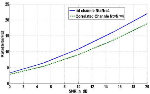
Fig. 7: Capacity reduction due to correlation of MIMO channels.

The result for iid (independent identically distributed) channel and correlated channel is shown in figure 7, it can be concluded form the figure, that in case of correlated MIMO channel, there is slight reduction in the channel capacity in comparison to iid channel. However, at lower SNR level the reduction is much less and can be neglected, but as the SNR increases the difference becomes significant.

• VII. Conclusions

In this paper, the channel capacity is estimated when CSI is known/not known at the transmitter, and it has been concluded that knowledge of the CSI at the transmitter is not a stringent requirement. This is also true in case of random MIMO channel, and it is concluded that then capacity is comparatively better in case of MIMO channel in compassion to others, and the capacity increases with N_T and N_R . The channel capacity for the random MIMO channels is also estimated through simulation. Finally, MIMO channel capacity in the presence of antenna correlation effect is estimated and it has been found that the capacity get reduced due to the correlation effect.