Error Measurement & its Impact on Bilateral -Canny Edge Detector-A Hybrid Filter

Автор: Sangita Roy, Sheli Sinha Chaudhuri

Журнал: International Journal of Modern Education and Computer Science (IJMECS) @ijmecs

Статья в выпуске: 2 vol.8, 2016 года.

Бесплатный доступ

Image Processing, a subset of Computer Vision, is an important branch in modern technology. Edge detection is a subset of segmentation to detect object of interest. Different image edge detection filters and their evaluating parameters are introducing rapidly. But the performance of an edge detector is an open problem. In this paper different performance measures of edge detection have been discussed in details and their application on a hybrid filter using Bilateral and Canny is proposed. Its parametric performance has been evaluated and other well established or classical existing edge detecting filters have been compared with it to measure its efficiency.

Еще

Bilateral Filter, Canny Edge Detector, Pratt Figure of Merit, Ems

Короткий адрес: https://sciup.org/15014837

IDR: 15014837

Текст научной статьи Error Measurement & its Impact on Bilateral -Canny Edge Detector-A Hybrid Filter

Published Online February 2016 in MECS DOI: 10.5815/ijmecs.2016.02.04

Automated Information System (AIS) is the buzz word in computer science. It is a collection of hardware, firmware, software or combination of all to perform a specific application like communication, data processing, storing etc. Objective as well as subjective evaluation is an integral part of any problem solving operation using Automated Information Processing. A comparative study of different measurement parameters of a given problem have been evaluated in this work. These parameters can be used as object functions in optimization. Through these assessments tuning and justifications are adjusted for different applications. Parameter tuning plays an important role in Machine learning. Machine learning is a subset of computer science which gradually developed from pattern recognition and computational learning theory of Artificial Intelligence. Object detection is an important branch of image processing, subset of computer vision. Application domains of object detection are face recognition, pedestrian detection, image retrieval, video surveillance, name a few. Therefore it is a challenging area. Edge detection in image processing is a subset of object detection. Optimum edge detection is an open problem and performance of an edge detector plays a significant role to determine how close the detector to the ideal one [45]. Objective measure is very important in case of edge detection [46]. This paper is organised as follows: review of error measurements in edge detection and classical filters, definition of edge in an image with different concepts, different errors in edge detection with mathematical concepts, experiments of those error metrices on standard bilateral and state-of-the art canny edge detector , and then the same process applied on hybrid filter . After that step comparative analysis of those three filters are carried out. Finally Bilaterl-Canny Edge detector has been found to be the better one in comparison with the other two counterparts from the point of view of their quantitative as well as qualitative analysis.

A. Literature Review in edge detection

Engineering education has evolved into the teaching of There are three categories of performance measurement in edge detection, i) quantitative, ii) qualitative, and iii) hybrid. Quantitative measurement is related with mathematical analysis, second one is associated with linguistics evaluation like human interaction, and it can’t be measured. Repeated surveys are time consuming and impose extra burden on a process for repeated evaluation. Moreover repeated evaluation by different human being makes the survey diverse [1]. Hybrid evaluation makes the presence of human users providing numerical evaluation of results [2, 3].But the said method is subjective, time consuming, and non-reproducible [4]. Qualitative and hybrid evaluation are not suitable because of human intervention that leads to inaccuracy. There are three basic difficulties in edge detection problems. i) How would edge image be formatted? ii) how would an perfect edge image be found? iii) How to compare two edge images? It is very difficult to define edge [5].

Edge detection is a demanding image analysis technique in image processing. In image analysis different intensity pixels are there and meaningful information have to be processed from the data set. Image segmentation separates meaningful data from the unnecessary data. Three different segmentation methods are broadly defined, namely a) Region growing and shrinking, b) clustering methods, and c) boundary methods. Region growing and shrinking method are operated on row and column of an image i.e., can be used in spatial domain. Boundary methods can be used in any domain. Edge detection can be said as a subset of boundary detection. Spatial Domain is of great importance in image processing [6]. Performance evaluation of an edge detector is quite a puzzling problem. There are two types of parametric evaluation namely a) objective, and b) subjective. Finally human is the best judge for the quality of an image and it changes from person to person and area of use. Therefore perception of human vision and analytical performance both are important in evaluating quality of processed images. Besides the existing edge detectors newer hybrid detectors are appearing with improved performance. Here authors examined extensively one hybrid filters along with classical filters like canny edge detector and bilateral filter. This hybrid filter is a hybridization of bilateral filter with canny edge detector. In 1986 J Canny proposed an edge detection method where he first detected an edge and then localized the edge delimiting multiple responses by non-maxima suppression [22, 23]. In 1995 Aurich et al. proposed non-linear Gaussian diffusion smoothing image filter by using modified heat conduction equation which is acquired by convolving initial data i.e., an image with Gaussian kernel. It is very simple as well as escapes iterative steps and convergence problems [24].Smith et al. in 1997 suggested Edge, and corner detection with structure preserving and noise minimization. Local image region of similar intensity around a pixel are identified, minimised, and smoothened by using non-linear filter. This method is noise resistant, fast and accurate [25]. C Tomasi, R Manduchi first described the name Bilateral Filter in 1998 which smoothens while preserving edges in images by nonlinear combination of nearby pixel values. It can be operated on both grey as well as colour images [26].In this paper authors have studied different EMs from literature. Then they synthesised and analysed the behaviour of those EMs on different benchmark and other simple images, specifically their quantification of errors on those given edge images using classical as well as one hybrid filter.

Table 1. Lists of Abbreviation Used

Sl. No.		EMs	Full Form
1.	Statistical EMs	Entropy	Amount of energy of an image
2.		Correlation	Relationship or similarity between two images
3.		PSNR	Peak Signal to noise ratio
4.		MSE	Mean Square Error
5.		MAXERR	Maximum absolute square deviation between two images
6.		L2RAT	Ratio of square norm of ground truth image to the candidate image
7.		PIXEL Count	Bright intensity pixels count i.e. edge pixels
8.		Egt	Ground Truth Image
9.		Ec	Candidate Image
10.		TP	True Positive(Hit)
11.		FP	False Negative(False alarm/ Type I error)
12.		FN	False Negative(Miss/ Type II error)
13.		TN	True Negative(Correct rejection)
14.		TPR	True Positive Rate
15.		BF	Ratio of FP to TP
16.		QP	Per cent ratio of TP to (TP+FP+FN)
17.		FPR	False Positive Rate
18.		ROC	Receiver Operating Characteristics
19.		Precision	Eq 11
20.		Recall	TPR
21.		FI	Eq12
22.		FI*
23.		KI	Eq 13
24.		F	Eq 14
25.	Distance based EMs	Average Distance DK	Average point-to-set distance
26.		Haralick DK	DK proposed by Haralick
27.		SDK	Symmetric distance function/ another version of DK
28.		HD	Hausdorff distance
29.		BDM	Baddeley’s Delta metric
30.		PFOM	Pratt Figure of Merit
31.		PFOM*	1-PFOM

B. What is an edge in an image?

Clear definition of an edge is absent due to its abstract nature. Haralick proposed a clear idea on an assumption that an image to be a continuous surface [7].It suggested an edge is a set of pixels whose intensity values change abruptly from the surroundings. Moreover author expressed high first derivative of f, where f is the function representing the image. Van Vliet et al. elaborated in a general way an edge to be a contour, centre of the slope with a good amount of gray level difference between the two regions [4].Some wobbly definition are there, like localization intensity change, sharp changes in intensity[8]. Strict definition of an edge depends on its application [19]. Finally it is observed that human experience is more fruitful than mathematical evaluation [20].Some author claims edge to be binary [21, 7]. Canny proposed widely recognised work [22, 23] by his optimal edge detector. Canny Edge Detector are characterised by i) Edge Detection, ii) Localization, iii) Non-maxima or multiple response Suppression iv) no spurious response. As the response is single the detected image is binary.

Low error rate (C1): edges that occur in the image should not be missed and there should be no spurious responses. Good localization (C2): the location of the edges should be as close as possible to their position in the image. Unicity(C3): each edge in the image should produce a single response.

C. Error in edge detection

It is now important to study error encountered in edge detection methods. There are commonly three kinds of errors. i) spurious responses (false positives, FPs), ii) missing edges (false negatives, FNs), and iii) displacements. For an edge detector it is not common for multiple responses for a single object boundary. FPs are associated with texture and noise. FNs are related with low contrast region. In case of image denoising excessive displacement of edges may occur from its true position. It has been found that displacement occurs with at least one FP and one FN, and it has been established that FP is quite closer to FN. In machine learning GT (Ground Truth) refers to a set of standard or benchmark or classical results, dataset or some standard objet which is or is used as a reference .GT (Ground Truth) is widely used in image processing.

D. Edge detection Evaluation

Desirable properties of an EM q where Egt is the ground truth image, E c is the candidate image.

i) Symmetry (E1): q (E c , E gt ) =q (E gt , E c )
ii) Single optimal solution (E2): q (E c , E gt ) =0<=> E gt =E c
iii) Sensitivity to degradation(E3): if р ∉ (Еgt ∪

E ), then q(E , ^Egt)∪(p), Egt).

iv) Sensitivity to improvement (E4): if р ∈ Еgt and р ∉ E , then q(E ,Egt)>q(E ⋃ (p), Egt) .

E. Quantitative Approach to Edge detection

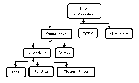
Fig.1. Error Measurement Hierarchy

There are three categories of performance measurement, i) quantitative, ii) qualitative, and iii) hybrid. Quantitative measurement is related with mathematical analysis, second one is associated with linguistics evaluation like human interaction, and it can’t be measured. Repeated surveys are time consuming and impose extra burden on a process for repeated evaluation.

Moreover repeated evaluation by different human being makes the survey diverse [1]. Hybrid evaluation makes the presence of human users providing numerical evaluation of results [2, 3].But the said method is subjective, time consuming, and non-reproducible [4]. Qualitative and hybrid evaluation are not suitable because of human intervention that leads to uncertainty. Ad Hoc EM is problem specific whereas generalistic EM assesses globally [10, 11]. Therefore AdHoc EMs can’t be useful for general purpose edge evaluation. Therefore generalistic EMs is the point of interest here. This can be subdivided into three i) local, ii) statistical, and iii) distance based. Local EMs checks properties of every edge pixel neighbouring for its regularity and continuity. This is a cumulative process and generates local information which leads to quality evaluation of edge image. One interesting and important criteria of Local EM with respect to any other EMs is that it does not require any ground truth. But it has one drawback that it can’t locate the exact location of edge [13]. Local EMs depict the good looks of an edge image, but unable to detect the accuracy of the edge image. But the above study does not mean that Local EMs are not useful. It is used for local features, like regularity, continuity which is worthy where true images are missing. Cost Function is a plot of cost vs. production in economics. It is widely used in edge detection minimization. An edge detection criterion consists of accurate localization, thinning, continuity and length. By using cost function between ground truth image and edge image minimization of edge have been found out. Edge detection is interpreted as a problem of cost minimization by using simulated annealing for optimization of five different EMs in the work of Tan et al. [9]. Local EMs cannot localize the exact edge location, due to this drawback it is not worthy for edge EMs [14, 8, 15-19].

F. Statistical edge measurement

Edge detection is a classification problem. In case of binary output it is a binary classification. The candidate edge image can be divided into four categories with respect to ground truth image, i) True Positive(TP), ii) True Negative(TN), iii) False Positive(FP), iv) False Negative(FN).It is evident that a very small portion of an image are edge pixels. Therefore an imbalance binary classification problem arises [27] where negative class dominates. Binary Classification problem is also known as binomial classification where class of data is divided into two groups. Example: medical test of a patient’s cancerous cell, pass or fail in the quality control in factory[c].When the data sets in binary classification problem become extremely unequal, then it is called unbalanced binary classification problem. Classification problem is the task of assigning a specific object to a class out of several predefined classes [28]. Spam or nonspam depends on the header and content of an email messages. Malignant or not also classify according the cell MRI scan. Classification of galaxies also depends on their shapes [28].Confusion Matrix is a branch of machine learning. It is also known as contingency table or error matrix. It reflects the algorithm performance by means of a table. In supervised learning it is known as confusion matrix whereas in unsupervised learning it is known as matching matrix. In a classification system it has been given to train and discriminate between cats, dogs, and rabbits. The confusion Table 2. will enumerate a visualization of the algorithm. In the algorithm there are 27 animals, out of these 8 cats, 6 dogs and 13 rabbits [29].

Table 2. Confusion Table

	Predicted Class
Actual Class		Cat	Dog	Rabbit
	Cat	5	3	0
	Dog	2	3	1
	Rabbit	0	2	11

Table 3. Basic Architecture of a Confusion Matrix

TP(True Positive)	FP(False Positive)
FN(False Negative)	TN(True Negative)

Table 4. Confusion Matrix of Table 2.

5 True positives(actual cats that were correctly classified as cats	2 false positives(dogs that were incorrectly labeled as cats
3 false negatives(cats that were incorrectly marked as dogs	17 true negatives(all the remaining animals , correctly classified as non-cats)

In edge detection edge pixels are very small in amount in comparison with the whole image. Therefore edge detection is imbalanced classification problem. A simple edge detection problem using confusion matrix is as shown below.

TP ^| ^EC ^∩ ^ESt ^|

FP=|EC ∩Eat| =

TN |Ec∩ Est | =

FN ₌ | — ^∩ ^ | | P |

All the operators have been used above as normal mathematical meaning.

Si (Egt, Ec)=|- ⊝| | v|

S2 (Egt, Ec)=|- | | ∖ ; | |

S, ( Egt , E,)= || ∩ | |

NSR ( Egt , Ec)=||I ⊝∩ Egt ||

S1 is the ratio of misclassified pixels. (S2, S3) is the ratio of edge/ non-edge pixels missed, and NSR is the ratio of the noise to signal. Statistical EMs have some shortcomings of spatial concerns i.e., FP closeness to actual edge pixels and regularity of the edges.P1 is the ratio between the number of points detected in the edges and those due to both the intensity transition and the noise. P2 is the percentage of rows covered by, at least, one edge point. These two measure hold good for specific images, rarely be used to other images [1]. Statistical EMs doesn’t compete fully with the canny constraints C1, C2, C3. Shortcomings of C1 tend to increment of FPs and FNs. Not satisfying C2 does not generate any change in FPs or FNs unless localization is perfect. Failing to the criteria C3 only increments FPs. To overcome these problems of statistical EMs, two statistical EMs are combined by receiver operating characteristic (ROC) plot [30, 31, 32, and 33]. True Positive Rate and False

Positive Rate are the two measures which are displayed in the ROC plot as the quality of an edge image.

TPR = =

TP+FN

FPR =

FP+TN

Alternative ROC plot can be evaluated by the Precision-Recall (PR) plots [34]. In this process TPR is denoted as recall and FPs are different, known as PREC where precision concept deploys.

Erec TP+FP (11)

BF = / TP

QP =100 ∗ TP /( TP + FP + FN )

Therefore PR plots employ eq (9) and (11) which are free from TN. This signifies that alternative PR plot is unaffected by true negative which in turn makes the evaluation more stable. This should be mention here that TN is much pronounced than its counterpart TP, FP, and FN. At the time of enlarging an image positive pixels increases linearly whereas negative pixels increases quadratically. The ROC and PR plot can be converted into their scalar and compatible version [33].

" E )_TP TN _ TPR ∙ TN

*gt , )^{= ∙ =}

It is a coefficient of evaluation of edge image using different thresholding procedures [35, 36].

Another evaluation coefficient is famous χ2 [37, 38].

z² ( Egt , E_c _{)= ∙} ( l-FPR )( ⁾ (13)

where Q=TP+FP.

Another measuring parameter is F measure [39].

Fa ( Egt , E_c )=

Prec ∙TPR aTPR +(1-a)Prec

where α ∈ [0,1] a weighing parameter according to precision-recall evaluations.Now is some interesting properties will be explored. As it has already been established that error measurement is the most important goal not its quality. Therefore compliment of equations (12), (13), and (14) are as follows:

∅∗(Egt, Ec)=1-∅(Egt, Ec)

Z2 ∗( Egt, Ec)=1-z2 (Egt, Ec)

Ft ∗( Egt, Ec)= 1-Fa (Egt, Ec)

∅^∗ ,χ² ^∗ ,F ^∗ Satisfy the basic properties E2, E3, E4. But E1 only embraces true for χ² ^∗ .Egt is a ground truth image. Ec1 and Ec2 are two candidate images for this EMs evaluation [reference fig 4]. In Ec1 one false negative is added whereas in Ec2 ten false positives are added. EMs q are quantified in the table 5.

Table 5

Measurement	∅ ^∗	z² ∗	F. ^∗.74	F. ^∗ .	F. ^∗.74
q(E gt , E c1 )	0.143	0.158	0.111	0.078	0.040
q(E gt , E c2 )	0.140	0.599	0.222	0.364	0.416

There are ten false positive points in EC2. But ∅^∗ is unresponsive to EC1 and EC2.Whereas other two parameters suffer from drastic changes. Statistical EMs depend on spatial tolerance i.e., the exact edge pixel located t or t+1 pixel away. A quality measure is precise if small changes in the detector output are reflected by small changes in its value [33]. This statement shows the light on distance based EMs.

G. Distance based Error Measurement

The distance-based EMs are established on the deviance of the edges from their true position [4], and studies the spatial location during evaluation. Its main objective is to fine an edge point consistently according to its distance from its actual point. Hence evaluation of an edge image is carried out as a mapping of distance to the ideal solution.

p 1 , ^p2 ∈ p ,be the position of an image, d(p1,p2)

denoted as Euclidean distance between them. d(p, E), where p∈Р and E∈ IE is an edge image , the distance from p to the nearest point p ∈ E, i. e., d(p, E) =min{d(p, p )|p ∈E} . Euclidian distance is the most widespread option, still few authors prefer to practice other benchmark distance functions like Chebyshev[40].Few EMs use average point-to-set distances[46, 7]. An average distance form edge pixel of the candidate image with respect to ground truth image

Dk (Egt, Ec)= √∑p∈ E^ (P, Egt)

wit ℎ к ∈ ℝ⁺

H(Egt, Ec)=|E ∪ ^ | ∑ peEc∩ Egt^(P, Egt)

_{( F} (∑ P ∈ Ec^ ⁽ P ^, Egt ⁾ ⁺ ^∑ P ∈ Egt^ ⁽ P ^, Ec )) "^k

DL>K (^t , ^c)=

(| Ec ∪ Egt |) ^k

PFoM ( Egt , Ec)= (|Egt|,|Ec|)∑P∈ Ec 1+k ∙d2 (p,Egt(21)

∆ ^kw ( Egt , E_c )=

[p∑p∈p|w.a(p, Egt)/-w(d(P, Ec))| ]

II. E xperiment of B ilateral -C anny H ybrid E dge D etector using EM s q (E rror M easurements )

A. Canny Edge Detector

Performance of Canny Edge Detection is optimum under step edges. The Canny Edge Algorithm:

Step 1. Smoothing – blurring of the image to remove noise by Gaussian Kernel.

Step 2. Finding the Gradients of edges and assigned where the gradient of the pixels are largest in magnitudes

Step 3. Non Maxima Suppression-local maxima intensity pixels are found to be edges.

Step 4. Double Thresholding – Eligible edges are determined by double thresholding

Step 5. Edge Tracking by Hysteresis-Finally edges are marked by strong continuous line.

Canny detector uses Gaussian filters in four directions-horizontal, vertical, and diagonal directions. The edge magnitude and direction can be determined by G and θ

G = √( Gx )2+(Gy )2

G=|Gx + Gy |

Gx and Gy are the gradients in x-direction and y-direction respectively. The direction of edge can be determined by e =tan -1 | ? |

| Gy |

After step one nonmaxima suppression is carried out where edge thinning is obtained. This results blurring of edges. Out of those blurred edges the brightest edge pixels are detected and the other pixels are reset to zero. After nonmaxima suppression there may be some spurious responses which may be due to noise and colour variation. These can be removed by keeping the highest gradient values while rejecting weak ones. After this stage there is double thresholding. Two threshold values are determined. If some edge pixels are above the threshold value, then they are definitely real edges. Those who are below the lower threshold are rejected. A lot of debate is on about whether the in between values are weak edges. Generally these weak edges are generated out of true edge extraction or noise or colour variation. Edge extracted pixels are recognized as edge and noise or colour variations pixels are rejected. Edge extracted pixels are connected to strong edge pixels by using BLOB (Binary Large OBject) Detection. BLOB gives complementary information about a region where edge detector fails. This step is known as hysteresis.

B. Bilateral Filter

Bilateral filter image can be defined as spatial domain, nonlinear, edge conserving and noise decreasing smoothing image filter. In this filter intensity value of each pixel is replaced by weighted average of its surrounding pixel values which is determined using Gaussian distribution not only by Euclidean distance of pixels but also by depth difference, colour intensity difference, and range difference. That is why sharp edges are preserved by symmetric looping of each pixel and correcting adjacent pixels accordingly.

jfi11ere 4 (^) = _L ^ _£ ^. )^ ( щ^ . ) -

I (x)Hk( Hx-xH) (27)

Where the normalization term

Wp = ^J_r (H/fc )-I (x)H)a_s Hx-xH ) (28)

I^fl itered (_x) is the filtered image. I is the original image. Wp is the normalised term.fr is the range kernel for smoothing differences in intensities (may be Gaussian Function).Gs is the spatial kernel for smoothing differences in coordinates (may be Gaussian Function).X is the coordinate of the current pixel to be filtered.Ω as given in eq(4) is the window centred to x (i, j) is the pixel of interest to be denoised in the image. (K, l) is the one of the neighbourhood pixels. The weight assigned to the pixel (k, l) to denoise the pixel (i, j) is given as

(i-fc)2+Q-ft)2 Ht(ij) -Z(fc,Z)H2

w ( i,j ,кД)= e ^{2 ff}d ^2ff2 (29)

σd and σr are smoothing parameters and I(i, j) and I(k, l) are the intensity of pixels (i,j) and (k,l) respectively. After calculating the weights, they are normalized.

_ ЕуТС^Ои/Силд)

= Z fc,z (i,7,k,i)

ID (i, j) is the denoised intensity of pixel (i, j). σr is the intensity or range control parameter and σd is the spatial control parameter for the filter kernels. By increasing these parameters, intensities and spatial domain features are smoothened respectively. Stair case effect like cartoon effect and gradient reversal i.e., false edge detection are the shortcoming of Bilateral filter.

III. Proposed Methodology

In edge detection hybrid or improved edge detector often gives little better results than that of the original filters. Here authors have developed a new hybrid edge detector where bilateral filter is acted upon canny edge detector.

Algorithm:

Step-I. Get Benchmark Input Image

Step-II. Bilateral Filter operated on the Image

Step-III. Canny Edge Detector operated on Step-II Step-IV. Get Output Image from Step-III.

Flow Chart:

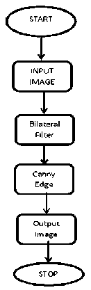
Fig.2. Flow Chart of New Methodology

A. Performance Evaluation

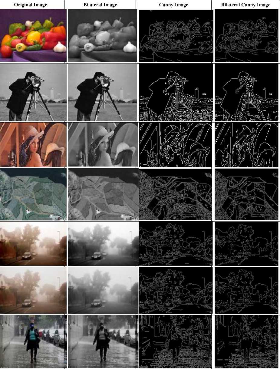
As it has already been stated that a new hybrid filter has been developed in this work. Here output of a bilateral filter has been passed through an Optimal Canny Edge Detector. To validate the new filter authors have evaluated its Parametric Performance. Some standard parametric performance has been tabulated using three standard benchmark images as well as four other images.

2) . Filtered Output

Subjective analyses have been given in the above tables. Its objective counterpart is being validated below. Table 11 shows perception of visual effects of original images and their Bilateral, Canny, and Hybrid output. These images are different in nature, e.g., human figure, human face, landscape, small lane as well as lane with mist, human in rain which gives a variety of contrast images. .Whereas in table 7-10 analytical outlook of those same images have been shown. In almost every case it is evident that pixel count of hybrid filtered images decreases whereas PFOM increases or are same in comparison with Canny which signifies that real edges are more pronounced in case of Bilateral Canny with lesser number of false edge detection. Image 5 and 6 are either foggy or dimmed. In these figures PFOMs are not improved by hybrid filter whereas false edges are removed as far as possible. PFOM increases in case of figure 7 which is a rainy image. At the same time according to the perception of vision object of interest are clearer in case of hybrid filtered images which is established by taking several human opinions. In table 8

3) . Statistical EMs

it has been shown by graphical representation. Therefore in all the above seven figures fewer edges are detected without losing the meaning of edge detection and object of interest. Therefore in all kind of images this proposed hybrid filter works well.

Table 6. Standard Benchmark Images with Their Entropy

Sl. No.	Benchmark Image	Entropy
1.	Peppers	7.3785
2.	Lena	7.525
3.	Cameraman	7.0097
4.	Aerial1	7.1779
5.	Car in a Lane	7.3723
6.	Car in a Lane with mist	7.5190
7.	Woman in Rain	7.4983

Table 7. Statistical Ems

Image: Pepper					Image: Cameraman
Sl. No.	EMs	Canny	Bilateral	Bilateral Canny	Sl. No.	EMs	Canny	Bilateral	Bilateral Canny
1.	Entropy	0.3581	6.9487	0.3127	1.	Entropy	0.4713	6.8866	0.3684
2.	Correlation	0.1146	0.9971	0.1036	2.	Correlation	0.0474	0.9950	0.0543
3.	PSNR	8.6743	8.7016	8.6731	3.	PSNR	5.5878	5.6164	5.5861
4.	MSE	8.8237e+03	8.7683e+03	8.8261e+03	4.	MSE	1.7960e+04	1.7842e+04	1.7967e+04
5.	MAXERR	255	254.0318	255	5.	MAXERR	253	252.0554	253
6.	L2RAT	7.6857e-06	1.5363e-05	6.3746e-06	6.	L2RAT	5.6022e-06	1.5302e-05	3.9297e-06
7.	Pixel Count	13354	54838	11222	7.	Pixel count	6602	48374	4631
8.	Time (s)	0.458482	14.943126	15.740298	8.	Time (s)	0.182248	3.656065	4.009621
9.	TPR	31.7733	71.5463	32.6930	9.	TPR	73.1785	99.1733	65.1279
10.	BF	6.6612	1.8524e-04	7.7087	10.	BF	7.0775	0.0025	9.8120
11.	QP	9.1396	71.5344	8.0717	11.	QP	9.7229	98.9279	5.9643
12.	FPR	6.6612	1.3927e-04	7.9251	12.	FPR	7.0775	0.0019	9.7227
13.	Precision	0.1091	0.9998	0.0949	13.	Precision	0.0996	0.9980	0.0620
14.	Recall	0.3177	0.7035	0.3345	14.	Recall	0.7318	0.9909	0.6532
15.	FI	0.3177	0.7173	0.3221	15.	FI	0.7318	0.9909	0.6602
16.	FI*	0.6823	0.2827	0.6779	16.	FI*	0.2682	0.0091	0.3398
17.	KI	0.3177	0.7163	0.3244	17.	KI	0.7318	0.9910	0.6560
18.	KI*	0.6823	0.2837	0.6756	18.	KI*	0.2682	0.0090	0.344
19.	F(0.25)	0.4318	3.8387	0.3794	19.	F(0.25)	0.3966	3.8744	0.2466
20.	F(0.5)	0.2174	1.9719	0.1847	20.	F(0.5)	0.1988	1.9763	0.1226
21.	F(.75)	0.1452	1.3268	0.1232	21.	F(.75)	0.1327	1.3261	0.0807
Image: Lena					Image: Aerial1
Sl. No.	EMs	Canny	Bilateral	Bilateral Canny	Sl. No.	EMs	Canny	Bilateral	Bilateral Canny
1.	Entropy	0.4857	7.0902	0.4204	1.	Entropy	0.5680	6.7678	0.4704
2.	Correlation	7.4574e-04	0.9889	0.0041	2.	Correlation	0.1160	0.9821	0.0860
3.	PSNR	7.7316	7.7575	7.8175	3.	PSNR	7.8205	7.8427	7.8176
4.	MSE	1.0963e+04	1.0898e+04	1.0967e+04	4.	MSE	1.0741e+04	1.0686e+04	1.0748e+04
5.	MAXERR	237	237.1804	237	5.	MAXERR	255	254.0792	255
6.	L2RAT	9.5909e-06	1.5246e-05	7.7627e-06	6.	L2RAT	1.2432e-05	1.5179e-05	9.3262e-06
7.	Pixel Count	5309	29030	4297	7.	Pixel count	30787	172950	23439
8.	Time (s)	0.156482	4.115834	4.303424	8.	Time (s)	0.520656	16.267749	16.776854
9.	TPR	29.6691	60.7175	28.9106	9.	TPR	77.4981	89.2524	74.8551
10.	BF	6.6409	7.7493e-05	7.9667	10.	BF	4.8365	7.5091e-04	6.4148
11.	QP	8.2587	60.7110	6.5176	11.	QP	14.9700	89.1916	10.9890
12.	FPR	6.6409	6.0834e-05	7.6765	12.	FPR	4.8365	4.8919e-04	6.5183
13.	Precision	0.0931	0.9998	0.0683	13.	Precision	0.1554	0.9992	0.1141
14.	Recall	0.2967	0.6089	0.2844	14.	Recall	0.7750	0.8922	0.7482
15.	FI	0.2967	0.6089	0.2982	15.	FI	0.7750	0.8883	0.7494
16.	FI*	0.7033	0.3911	0.7018	16.	FI*	0.2250	0.1117	0.2506
17.	KI	0.2967	0.6074	0.2971	17.	KI	0.7750	0.8927	0.7495
18	KI*	0.7033	0.3926	0.7029	18.	KI*	0.2250	0.1073	0.2505
19.	F(0.25)	0.3690	3.8108	0.2747	19.	F(0.25)	0.6180	3.8669	0.4484
20.	F(0.5)	0.1856	1.9675	0.1358	20.	F(0.5)	0.3102	1.9762	0.2238
21.	F(.75)	0.1240	1.3260	0.0925	21.	F(.75)	0.2071	1.3274	0.1504

Image: Car in a Lane					Image: Car I a Lane with mist
Sl. No.	EMs	Canny	Bilateral	Bilateral Canny	Sl. No.	EMs	Canny	Bilateral	Bilateral Canny
1.	Entropy	0.3546	7.6566	0.2578	1.	Entropy	0.3568	7.4205	0.2696
2.	Correlation	0.0576	0.9993	0.0368	2.	Correlation	0.0611	0.9991	0.0412
3.	PSNR	3.9101	3.9415	3.9092	3.	PSNR	4.3380	4.3691	4.3371
4.	MSE	2.6428e+04	2.6238e+04	2.6434e+04	4.	MSE	2.3948e+04	2.3778e+04	2.3954e+04
5.	MAXERR	255	254.0280	255	5.	MAXERR	234	233.1000	234
6.	L2RAT	2.5338e-06	1.5316e-05	1.6426e-06	6.	L2RAT	2.8195e-06	1.5377e-05	1.9239e-06
7.	Pixel Count	15438	117880	10008	7.	Pixel Count	15568	118240	10623
9.	Time (s)	0.369753	16.012605	16.382358	9.	Time (s)	0.334783	14.688716	15.23499
10.	TPR	43.8537	99.6880	45.6370	10.	TPR	43.6213	99.6957	45.9964
11.	BF	11.2238	0.0076	15.1957	11.	BF	11.2357	0.0100	15.6300
12.	QP	5.4461	98.9212	3.8537	12.	QP	5.3880	98.6777	3.7832
13.	FPR	11.2238	0.0079	15.2860	13.	FPR	11.2357	0.0096	14.9373
14.	Precision	0.0575	0.9920	0.399	14.	Precision	0.0397	0.9903	0.0569
15.	Recall	0.4385	0.9969	0.4751	15.	Recall	0.4549	0.9969	0.4362
16.	FI	0.4385	0.9968	0.4737	16.	FI	0.4362	0.9967	0.4522
17.	KI	0.4385	0.9968	0.4657	17.	KI	0.4362	0.9973	0.4611
18.	KI*	0.5615	0.0032	0.5343	18.	KI*	0.5638	0.0027	0.5389
19.	F(0.25)	0.2290	3.8638	0.1600	19.	F(0.25)	0.2266	3.8464	0.1630
20.	F(0.5)	0.1148	1.9651	0.0785	20.	F(0.5)	0.0758	1.3160	0.0786
21.	F(0.75)	0.0766	1.3181	0.0536	21.	F(0.75)	0.0569	0.9901	0.0540
Image: Woman in Rain
Sl. No.	EMs	Canny	Bilateral	Bilateral Canny	Sl. No.	EMs	Canny	Bilateral	Bilateral Canny
1.	Entropy	0.4985	7.4693	0.4138	11.	QP	10.2862	94.1000	7.2919
2.	Correlation	0.0338	0.9922	0.0197	12.	FPR	5.8427	0.0136	7.4542
3.	PSNR	6.9373	6.9635	6.9354	13.	Precision	0.1062	0.9862	0.0738
4.	MSE	1.3163e+04	1.3084e+04	1.3169e+04	14.	Recall	0.5767	0.9542	0.5412
5.	MAXERR	255	254.1036	255	15.	FI	0.5767	0.9544	0.5413
6.	L2RAT	8.3053e-06	1.5217e-05	6.3201e-06	16.	KI	0.5767	0.9539	0.5419
7.	Pixel Count	29905	156302	22757	17.	KI*	0.4233	0.0461	0.4581
8.	Time (s)	0.334783	17.206897	17.541680	18.	F(0.25)	0.4225	3.8256	0.2988
9.	TPR	57.6703	95.4275	54.0619	19.	F(0.5)	0.2120	1.9516	0.1523
10.	BF	5.8427	0.0139	7.3729	20.	F(0.75)	0.1415	1.3109	0.0968

Table 8. Plot of Statistical Ems q

Sl. No.	EMs	Plot	Sl. No.	EMs	Plot
1.	Entropy	N 6 — P ■ -► Bilateral V//z	8.	BF	20 — is— В д \ ¹⁰ " \\--Саппу F ₅ • _________ ^в—Bilateral
2.	Correlation	! ^ол -■- Bilateral a 0,2--—e—Hybrid । 0 *^-~^^	9.	QP	⁸⁰ Q 60 —♦ Саппу ⁴⁰ -^Bilateral ²⁰ д ^ д,-»- ^ ^ ^ .--Hybrid XZ^v
3.	PSNR	N а —«—Саппу R 3 —■—Ullatwal	10.	FPR	20 15 - — F10 ..д. /X “♦“Слипу Р ₅ -•-Bilateral о ■l■l■l■l■l■l■ ^^№И XZV/ ^'Х
4.	L2RAT	1.6ОЕ-О5 ■ ■ р ■ Н ■ ■ _R 8.00Е 06 ^- /л'\\ X * Саппу д 600Е-06 ^Vz Vl X* -^Bilateral Т 4XDE-06---- —е—Hybrid O.OOEiQO -------1---------------г-------г-------г-------г-------1 ^q У У	11.	Precision	Р 0.6 ------------------------------------- • Саппу _е °-⁴ ^-Bilateral С ^{0 2} > д ф-^^-^ д ^ -Д ——Hybrid /Z^/^//

Pixel Count

200000 п----

Р ■

| 150000 ------ -Д

* 100000 --/---------—*—Саппу

L 50000 ^-Ж^/ ---- —■—Bilateral

^н Ybr id

/УУ^ У"

12.

Recall

c ⁰⁶ -*-canny

^{a 04 B} * -«-Bilateral

^0,2 —e—Hybrid

ZZ^zZ

TPR

р4О , / \/ ^ ***♦-Bil atera 1

R²q a Hybrid

Z/у/ ^ ^ ' V'

13.

‘«^Mмоем . _e щсян

* Уу ^z X * Z/

F(0.25)

2 i I Canny

14.

F(0.5)

У у Z Z ^' X X

4) . Distance Based EMs

Table 9. Distance Based Ems

Image: Peppers					Image: Cameraman
Sl. No.	EMs	Canny	Bilateral	Bilateral Canny	Sl. No.	EMs	Canny	Bilateral	Bilateral Canny
1.	PFoM	0.8563	0.7267	0.8424	1.	PFoM	0.8757	0.7678	0.8788
2.	PFoM*	0.1437	0.2733	0.1576	2.	PFoM*	0.1243	0.2322	0.1212
3.	HD	15.0333	11.7047	14.9332	3.	BDM	26.4701	0.1928	26.5544
4.	BDM	19.3050	8.8822	14.1190	4.	HD	12.4900	5.3852	13.6748
Image: Lena					Image: Aerial1
Sl. No.	EMs	Canny	Bilateral	Bilateral Canny	Sl. No.	EMs	Canny	Bilateral	Bilateral Canny
1.	PFoM	0.8581	0.7363	0.8647	1.	PFoM	0.8840	0.6654	0.8009
2.	PFoM*	0.1419	0.2637	0.1353	2.	PFoM*	0.1159	0.3346	0.1991
3.	BDM	5.4565	3.6568	6.5517	3.	BDM	4.3942	0.4270	6.1752
4.	HD	12	10.0995	11.9583	4.	HD	20.4450	10.3923	20.7846
Image: Car in a Lane					Image: Car in a Lane with mist
Sl. No.	EMs	Canny	Bilateral	Bilateral Canny	Sl. No.	EMs	Canny	Bilateral	Bilateral Canny
1.	PFoM	0.8486	0.4960	0.7371	1.	PFoM	0.8534	0.5307	0.7463
2.	PFoM*	0.1514	0.504	0.2629	2.	PFoM*	0.1466	0.4693	0.2537
3.	BDM	47.4500	5.3654	45.8977	3.	BDM	47.2729	7.4160	45.6978
4.	HD	22.5167	6.7082	23.1948	4.	HD	22.8254	6.8557	23.7697
Image: Woman in Rain
Sl. No.	EMs	Canny	Bilateral	Bilateral Canny	Sl. No.	EMs	Canny	Bilateral	Bilateral Canny
1.	PFoM	0.8558	0.7063	0.8626	3.	BDM	6.9423	1.4940	9.9340
2.	PFoM*	0.1442	0.2937	0.1374	4.	HD	19.3907	9.0554	19.5704

Table 10. Plot of Distance Based Ems q

Sl. No.

EMs

Plot

Sl. No.

EMs

Plot

PFoM

8.00E-01 _ _H

F 6.0OEO1 --------------- X,----- /*--

0 5.00E-01--«■"■----

M 4.00E-01 --------------------------------- -^Cann,

3.00E-01 -И-Bilateral

2Л0Е01 --------------------------------- -4-Hytrid

^/^/^^z

PFoM*

\ —*—^Canr*v

\ / V-«-Bilateral

° f Ж-^*х^^*— Hybrid

BDM

D _M . \к--- -f- Canny

^M IS —1^---V-----7---------V— -«-Bilateral

H ■ Z ^{1 1} Canny

~ -■-Bilateral

Table 11. Visual Output of Different Original and Their Filtered Images

Sl.

Original Image

Bilateral Image

Canny Image

Bilateral Canny Image

Список литературы Error Measurement & its Impact on Bilateral -Canny Edge Detector-A Hybrid Filter

H. Nachlieli, D. Shaked, Measuring the quality of quality measures, IEEE Transactions on Image Processing 20 (1) (2011) 76–87.
M. Heath, S. Sarkar, T. Sanocki, K. Bowyer, A robust visual method for assessing the relative performance of edge-detection algorithms, IEEE Transactions on Pattern Analysis and Machine Intelligence 19 (12) (1997) 1338–1359.
M.Heath, S.Sarkar, T.Sanocki, K.Bowyer, Comparison of edge detectors—a Methodology and initial study, Computer Vision and Image Understanding 69 (1) (1998)38–54.
L. Van Vliet, I. Young, A nonlinear Laplace operator as edge detector in noisy images, Computer Vision Graphics and Image Processing 45 (2) (1989) 167–195.
C. Lopez-Molina, B. De Baets, H. Bustince, Quantitative error measures for edge detection, Pattern Recognition 46 (2013) 1125–1139.
S Roy, S S Chaudhuri, Performance Improvement of Bilateral Filter using Canny Edge Detection-A Hybrid Filter.
R.M. Haralick, Digital step edges from zero crossing of second directional derivatives, IEEE Transactions on Pattern Analysis and Machine Intelligence 6 (1) (1984) 58–68.
S. Coleman, B. Scotney, S. Suganthan, Edge detecting for range data using Laplacian operators, IEEE Transactions on Image Processing 19 (11) (2010) 2814–2824.
H. Tan, S. Gelfand, E. Delp, A cost minimization approach to edge detection using simulated annealing, IEEE Transactions on Pattern Analysis and Machine Intelligence 14 (1) (1992) 3–18.
M. Shin, D. Goldgof, K. Bowyer, S. Nikiforou, Comparison of edge detection algorithms using a structure from motion task, IEEE Transactions on Systems, Man, and Cybernetics, Part B: Cybernetics 31 (4) (2001) 589–601.
G. Liu, R.M. Haralick, Optimal matching problem in detection and recognition performance evaluation, Pattern Recognition 35 (10) (2002) 2125–2139.
T. Nguyen, D. Ziou, Contextual and non-contextual performance evaluation of edge detectors, Pattern Recognition Letters 21 (9) (2000) 805–816.
L. Kitchen, A. Rosenfeld, Edge evaluation using local edge coherence, IEEE Transactions on Systems, Man and Cybernetics 11 (9) (1981) 597–605.
S.M. Bhandarkar, Y. Zhang, W.D. Potter, An edge detection technique using genetic algorithm-based optimization, Pattern Recognition 27 (9) (1994) 1159–1180.
M. Gudmundsson, E. El-Kwae, M. Kabuka, Edge detection in medical images using a genetic algorithm, IEEE Transactions on Medical Imaging 17 (3) (1998) 469–474.
M. Kass, A.P. Witkin, D. Terzopoulos, Snakes: active contour models, Inter- national Journal of Computer Vision 4 (1988) 321–331.
V. Caselles, F. Catte′, T. Coll, F. Dibos, A geometric model for active contours in image processing, Numerische Mathematik 66 (1993) 1–31.
T. Chan, L. Vese, Active contours without edges, IEEE Transactions on Image Processing 10 (2) (2001) 266–277.
M Basu, Gaussian based edge detection methods- a survey, IEEE Transactions on Systems, Man, and Cybernetics, Part C: Applications and Reviews 32(3) (2002) 252-260.
G. Papari, N. Petkov, Edge and line oriented contour detection: state of the art, Image and Vision Computing 29 (2–3) (2011) 79–103.
J. Fram, E.S. Deutsch, Quantitative evaluation of edge detection algorithms and their comparison with human performance, IEEE Transactions on Computers C 24 (6) (1975) 616–628.
J. Canny, Finding edges and lines in images, Technical Report, Massachusetts Institute of Technology, Cambridge, MA, USA, 1983.
J. Canny, A computational approach to edge detection, IEEE Transactions on Pattern Analysis and Machine Intelligence 8 (6) (1986) 679–698.
Volker Aurich, Jörg Weule, Non-Linear Gaussian Filters Performing Edge Preserving Diffusion, Springer-Verlag Berlin Heidelberg.
S M Smith, J M Brady, "SUSAN- A New Approach to Low Level Image Processing, International Journal of Computer Vision, V-23(1), 45-78, 1997.Springer, DOI:10.1023/A:1007963824710.
C Tomasi, R Manduchi, Billateral Filtering for Gray and Color Image, Proceedings of IEEE International Conference of Computer Vision, Bombay, India, 1998.
N.V. Chawla, N. Japkowicz, P. Drive, Editorial: special issue on learning from imbalanced data sets, ACM SIGKDD Explorations Newsletter 6 (1) (2004) 1–6.
http://www-users.cs.umn.edu/~kumar/dmbook/ch4.pdf
https://en.wikipedia.org/wiki/Confusion_matrix
K. Bowyer, C. Kranenburg, S. Dougherty, Edge detector evaluation using empirical ROC curves, Computer Vision and Image Understanding 84 (1) (2001) 77–103.
Y. Yitzhaky, E. Peli, A method for objective edge detection evaluation and detector parameter selection, IEEE Transactions on Pattern Analysis and Machine Intelligence 25 (8) (2003) 1027–1033.
T. Fawcett, An introduction to ROC analysis, Pattern Recognition Letters 27 (8) (2006) 861–874.
W. Waegeman, B. De Baets, L. Boullart, ROC analysis in ordinal regression learning, Pattern Recognition Letters 29 (1) (2008) 1–9.
D. Martin, C. Fowlkes, J. Malik, Learning to detect natural image boundaries using local brightness, color, and texture cues, IEEE Transactions on Pattern Analysis and Machine Intelligence 26 (5) (2004) 530–549.
S. Venkatesh, P.L. Rosin, Dynamic threshold determination by local and global edge evaluation, Graphical Models and Image Processing 57 (2) (1995) 146–160.
P.L. Rosin, Edges: saliency measures and automatic thresholding, Machine Vision and Applications 9 (1997) 139–159.
R. Koren, Y. Yitzhaky, Automatic selection of edge detector parameters based on spatial and statistical measures, Computer Vision and Image Under- standing 102 (2) (2006) 204–213.
Y. Yitzhaky, E. Peli, A method for objective edge detection evaluation and detector parameter selection, IEEE Transactions on Pattern Analysis and Machine Intelligence 25 (8) (2003) 1027–1033.
D. Martin, C. Fowlkes, J. Malik, Learning to detect natural image boundaries using local brightness, color, and texture cues, IEEE Transactions on Pattern Analysis and Machine Intelligence 26 (5) (2004) 530–549.
M. Segui Prieto, A. Allen, A similarity metric for edge images, IEEE Transac- tions on Pattern Analysis and Machine Intelligence 25 (10) (2003) 1265–1273.
S Paris, P Kornprobst, J Tumblin, F Durand, A Gentle Introduction to Bilateral Filtering & its applications.
J Chen, S Paris, F Durand, Real-time edge-aware image processing with the bilateral grid, ACM Transaction on Graphics, 26(3), 2007, proceedings of the SIGGRAPH Conference.
W K Pratt, Digital Image Processing, PIKS Inside, 3rd Edition Wiley, 2001.
R C Gonzalez, R E Woods, Digital Image Processing, 3rd Edition, PHI.
J. Fram, E.S. Deutsch, Quantitative evaluation of edge detection algorithms and their comparison with human performance, IEEE Transactions on Computers C 24 (6) (1975) 616–628.
R.C.Jain, T.O.Binford, Ignorance, myopia, and naivete′ in computer vision.

Еще

Статья научная