Errors reduction while locating objects of the radio navigation system

Despite the significant progress achieved in the field of coordinate-time support using satellite radio navigation systems (SRNS), ground-based radio navigation systems (RNS) continue to play an important role in the coordinate support of aviation objects, ground vehicles and sea-based objects.

Currently, increased requirements are imposed on ground-based RNS due to the accuracy and reliability of radio navigation determinations, in addition, RNS should solve the problems of ground support for SRNS consumers. Such support can be implemented by assigning to the RNS the functions of transmitting differential corrections to the SRNS signals, this is implemented by placing SRNS control and correction stations (CCS) as part of the fixed stations (FS) of the RNS. In this case, the selected structure of the RNS signals should transmit blocks of digital information as a part of the navigation signals, carrying differential correction data and service messages at a given rate.

Reducing the error of radio navigation determinations in the RNS is impossible without solving another problem - synchronization of the time scales (TS) of reference stations, which ensures the setting of a unified system time scale (USTS) of the radio navigation system.

Currently, the ground-based RNS have to meet the increased requirements to the accuracy and reliability of radio navigation determinations, besides, RNS should contribute to solving the problems of ground support for SRNS consumers. Such support can be implemented by assigning to the RNS the functions of transmitting differential corrections to the SRNS signals, which is realized by placing

SRNS control and correction stations (CCS) as part of the fixed stations (FS) of the RNS. In this occasion, the selected structure of the RNS signals should transmit blocks of digital information as a part of the navigation signals, carrying differential correction data and service messages at a given rate.

Reducing the error of radio navigation determinations in the RNS is impossible without solving another problem - synchronization of the time scales (TS) of reference stations, which ensures the setting of a unified system time scale (USTS) of the radio navigation system.

Synchronization methods for reference stations of radio navigation systems

We consider the known methods to implement the system time scale in SRNS and RNS. For the SRNS GLONASS and GPS, implementing the USTS is performed by installing high-precision frequency and time standards on board each of the navigation spacecraft (NSC) and determining the parameters of the time scale drift of the NSС based on the measurement results performed by the stations of the ground control complex (GCC). Information about the values of the correction coefficients of the polynomials approximating the clock drift is put on board the SRNS navigation spacecraft from the GCC transmitting stations via a dedicated radio channel [1].

In the RNS, to implement a unified STS, the following methods can be used:

• 1)    RNS differential mode, requiring a control point (CP) located at a point with coordinates known in advance. In this case, the CP measurement results are used to calculate error corrections for each of the reference stations to STS. The obtained values of the error corrections for each of the reference stations to the STS are transmitted through a dedicated radio channel on the air. RNS consumers measure the values of radio navigation parameters and receive CP signals that carry information about corrections to FS (fixed station) time scales or to the values of radio navigation parameters (RNP). Using the received corrective information, the consumer corrects the results of their own measurements, due to that the errors caused by the FS time scale mismatch, as well as the correlated error components on the signal propagation path are eliminated [2];

• 2)    use of highly stable quantum frequency standards as part of the FS and the use of portable frequency standards for periodic comparisons of the FS time scales and the introduction of corrections to the STS [3; 4];

• 3)    RNS calibration according to the methods of FS mutual control and according to measurements at the control point [2].

The first method is realized by determining the values of error corrections based on the mutual control of the FS signals and inputting the resulting corrections into signals of each FC. The second method is implemented by determining the corrections to the signals of all FS RNS at the control point with certain coordinates, after which the value corrections obtained during the calibration are introduced into the composition of the emitted FS signals;

• 4)    RNS synchronization based on the use of external sources, for example, SRNS.

Disadvantages of existing methods to synchronize radio navigation systems

The existing methods for synchronizing the signals of RNS navigation points have the following disadvantages:

• –    the differential method of introducing corrections obtains a drawback, due to its need to allocate a special radio channel to transmit corrections in real time, CP organization and service, development of RNS consumer equipment, taking into account the need to receive additional signals emitted by the CP;

• –    the second synchronization method requires the availability of a portable frequency standard, the organization of transportation of this standard among the system stations, the comparison of time scales of the portable standard and FS frequency standards;

• –    the third method disadvantage is in the requirement to remove the RNS from the normal mode during calibration, which leads to interruption in providing consumers with information about the coordinates. In addition, within the time since the last calibration, information about the corrections becomes obsolete, due to the mutual discrepancy between the fixed stations' TS, due to the long-term instability of the frequency

of the used frequency and time standards, which leads to a gradual degradation of the accuracy of the determinations;

• –    the implementation of the fourth method is possible only if SRNS signals are received. But one of the SRNS features is the dependence of the RNP measurement accuracy on solar activity [5]. Moreover, RNS loses its autonomy if it is synchronized with SRNS.

The availability of these disadvantages is an incentive to develop a method for the formation of a unified system time scale and its correction by means of fixed stations of the ground-based RNS, which makes it possible to significantly reduce the impact of these disadvantages on the accuracy of measuring radio navigation parameters.

FS Time Scale Divergence Calculation Method

Fig.1 presents RNS geometric structure. The antennas of the transmitting devices of the fixed stations ОС А (is the leading fixed station), ОС B and ОС C (they are slave fixed stations) located at points A, B and C with coordinates known with geodetic accuracy ( xy ), ( xy ) and ( xy ), emitting radio navigation signals. Point M is the location of a board station (BS), the location (coordinates x _M y _M ) of which should be determined. Taking into account the certain moments of signal emission by the fixed stations (ОС А , ОС B and ОС C ) and the measured propagation times of the emitted radio navigation signals (primary processing of radio navigation signals [6]) at certain speeds of propagation of electromagnetic waves along the AM, BM and CM paths by means of equipment (secondary processing of radio navigation signals signals [6]) of the board station, the distances are determined, d_AM and d_CM of the paths AM, BM and CM, and the coordinates of the BS location are determined from the certain coordinates x_My_M of points A, B and C.

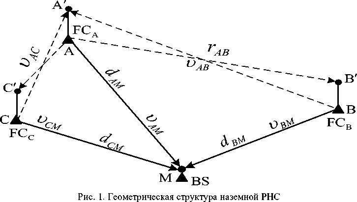
Fig. 1. Geometric structure of the ground-based RNS

The navigation system uses wideband signals with minimum frequency shift keying [7] (hereinafter referred to as signals), which narrow the baseband of the signal spectrum, reduce the level of side components, and also eliminate the need for a special radio channel to transmit the necessary information through the use of additional code phase shift keying (PSK). In this case, the most effective way to separate wideband signals emitted by fixed stations is the code method to separate such signals at the receiving side. The code signal separation method provides for the formation and emission of signals modulated by codes of pseudo-random sequences (PRS). If the PRS [8] is selected as the modulating code on the ОСА, then on the OСВ (OСС) cyclic shifts on nB (nC ) of binary symbols of the same original code PRS selected on the OCa are used as the modulating code PRS. If three signals are necessary to use, then the cyclic shift for each of the OC is defined as ni ≈(i-1)L/ j (here i is a number of a j fixed station; L = 2m - 1- the length of the original M-code of the PRS, generated by an mbit shift register, covered by feedback through the EXCLUSIVE-OR circuit). It should be added that when working with code signal division, all OC operate at the same frequency, and the emitted OC signals are overlapped in time.

Each of the OC includes both a transmitting and receiving device. The transmitting device generates and emits a signal through the radiating antenna. The receiving device receives and processes signals emitted by neighboring OC. The primary processing of the received signal will result in generating the the signal reception moment, taking into account the delay associated with the signal group delay in the high-frequency path and the delay due to tracking systems for the code delay and the phase of the radio signal [9]. A shortened asymmetric vertical antenna is used as a receiving antenna (with phase centers at points A′, B ′ and C′ ) of the fixed station; a shortened asymmetric vertical antenna locates with a vertical spacing of 1 m relative to the top of the emitting antenna (with phase centers at points A, B and C), which creates an isolation relative to the emitting antennas not less than 20 dB [10]. Besides, additional decoupling is provided by using the code division of the emitted signal sA(t,di) (di -PRS modulation code) by the OCa fixed station and the received signal sB(t-тр, din) (din - PRS modulation code with n cyclic shift) from the OCb fixed station. The value тр of the EMW propagation delay on the AB path is determined by the и AB propagation velocity of the surface electromagnetic wave in free space [11] and the selected distance rAB between the fixed stations. In this occasion, code division involves the calculation of the value of the signal cross-correlation sA(t,di) and sB (t - тр, din) . As shown above, the second signal differs from the first one by the modulating code corresponding to a cyclic shift by n binary symbols, and then it is necessary to calculate the autocorrelation value of the signals sA (t, di) and sB (t - тр, din) with their relative delay т = тР + nтэ (тэ - is symbol duration in the PRS code). It is also necessary to take into account the use of additional PSK code to these signals. According to the formulae [12] for the MFSK signal with a modulating M-code of the PRS of length L = 214 -1 = 16383 and with additional PSKM, a plot of the modulus of the normalized periodic (T = Lтэ - period) autocorrelation function (PACF) on the relative delay number k (k = [т/тэ]- an integer number of shifts per symbol PSP duration). Fig. 2 shows a segment plot (in order to obtain high resolution) of the modulus of the normalized PACF with PSKM over the interval [5308, 5476] of the shift number. Fig 2 demonstrates the delay 5398тэ could result in the minimum value – 1/L 10-4 . If the reference stations are at a distance of rAB =300 km from each other, then the signal propagation delay will be тр  1 m/s (using the speed uab 03 ’10 m/s, we make an error of 0.1% order) and at т э = 2,5'10 this will correspond to a delay of 400 PRS binary symbols. According to fig. 2, in order to provide the minimum value of the modulus of the normalized PACF (for k = 5398), it is necessary to use the modulating PRS code of the fixed station OCB with a cyclic shift of nB = 4998 = 5398 – 400 symbols. It can be mentioned that the signals sA(t,di) and sB (t - т р, din ) at the point of their processing (as well as at points belonging to the surface of a circle with т э U AB /2 ≈350 m radius, with the center of the receiving-radiating antenna) will be significantly separated, that is equivalent to providing additional antenna decoupling of no more than -42 db 10lg(1/L).

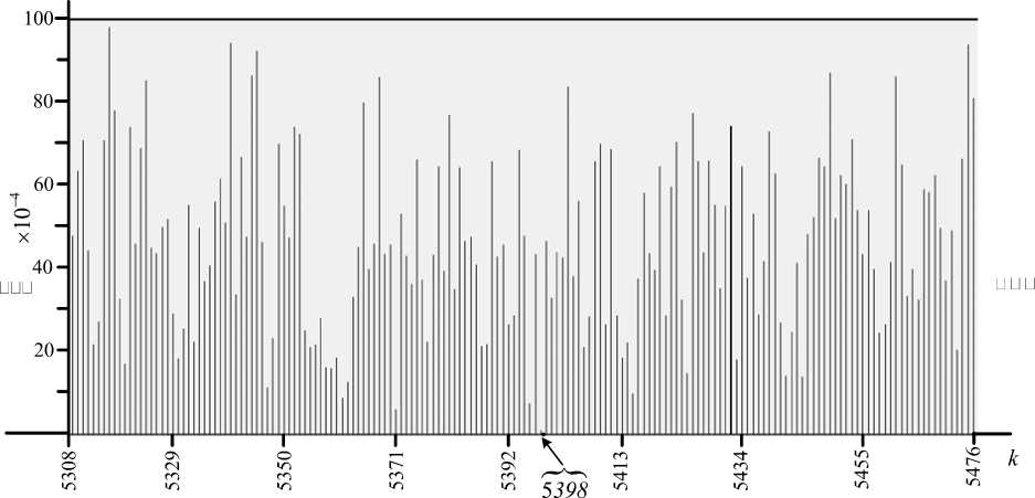
Рис. 2. Фрагмент модуля нормированной ПАКФ для МЧМ сигналов с дополнительной ФМ

Fig. 2. Fragment of the normalized PACF module for MFSK signals with additional PSKM

Fig. 3 shows time diagrams corresponding to the moments of reception and emission of RNS signals with the current time scales (TS*).

The time scale of every OC is a continuous sequence of intervals equal to L τ_э signal duration, counted from the point beginning of t = 0 time. Time scales which initial phases and complex signal envelopes coincide with the required accuracy at any interval of the signal duration are called synchronous [2] and during the measurement of navigation parameters it is necessary to maintain this synchronism. In our case, at time points t _A , t_B and t_C , the fixed stations OC a , OC b and OC c emit radio signals relative to their own time scales (TS А , TS В , TS С ) and time points t _* are not equal to zero. This happens due to the fact that in the inertial circuits of the formation of a high-frequency signal, a group delay occurs, which leads to a delay in the moment of emission of the "given" phase of the modulating code relative to the moment of its formation in the code generator and, accordingly, to the difference in the actual moment of radiation relative to that transmitted in the navigation message [13]. Connected to the identity of generating the radio signal shapers, this time is similar to all OC, that is t A = t B = t C relative to their own time scales (TS a , TS b , TS c ).

Relative to the TS a time scale of the OC a fixed station, the points t_A B and t AC arrival time of the signals are determined, when they are emitted by ОС В and ОС С fixed stations at the time points t_B and t C relative to the own time scales TS b and TS c [9]. The arrival time t B ‘ A of the signal emitted by the ОС A fixed station at the time t_A due to its own TS А time scale is determined; it happens relative to the TS b time scale of the ОС в fixed station. Regarding TS c time scale of ОС с fixed station, time point t C ‘ A is defined for the arrival signal emitted by ОС А fixed station at the time point t_A relative their own time scale TS А . In reference to time scale TS М of board station BS, time points t_MA , t_MC and t_MB for the arriving signals, when they are emitted by fixed stations ОС А , ОС С and ОС В at time points t_A , t_C and t_B regarding their own time scales TS А , TS С and TS В .

ST B

ST А

Δ t _B

t _A    t

CA'

BA'

t

t

AB'

tB

t B ' A

t

ST

AC'

ST M

Δ t_M

tC

t

t

τ _BM

^τ CM

τ AM

— —AM

CM

BM

tMA   tMC tMB

Рис. 3. Временные диаграммы приёма и передачи сигналов РНС

Fig. 3. Time diagrams of receiving and transmitting RNS signals

The signal propagation time τ _{AB ′} from point A to point B ′ is defined as τ _′ = r _′ / υ _′ (here r _′ - is the geographical distance between the fixed stations OC a and OC b , known with geodetic accuracy; υ _′ - is the propagation speed of an electromagnetic wave (EMW) along the path AB ′ ). In terrestrial RNS, the measurement of navigation parameters is carried out by measuring the propagation delay of the surface EMW. Here the EMW propagation velocity will depend both on the environmental parameters (temperature, humidity, pressure) and on the parameters of the near-surface layer of the EMW propagation area (dielectric and magnetic permeability, conductivity). Accurately predicting the values of all these parameters at the time of surface EMW propagation is practically impossible. Therefore, it does not matter how accurately we measure time τ _′ [14], it will always contain a random component Δτ _{AB ′} , conditioned by the variability in time of EMW propagation path parameters (when calculating distances, this will lead to an error due to the use of the calculated speed value instead of the actual speed υ _′ ). In accordance with this, the measured EMW propagation delay on the path can be represented as the sum of the exact delay value τˆ _′ and the error Δτ _′ in the form τ _{AB ′} = τˆ _{AB ′} + Δτ _{AB ′} .

Taking into account the above for the signal propagation time on the path BA ′ , the delay on the path BA ′ can be represented as the sum of the exact delay value τˆ _′ and the error Δτ _{BA ′} in the form τ _{BA ′} = τˆ _{BA ′} + Δτ _{BA ′} .

On the TS В time scale (Fig. 3) with respect to the time point t_B , it is possible to measure a pseudodelay [9] of signal propagation along the path AB ′ as

τ^*_B = t_AB ′ - t_B + Δτ _AB ′ = τˆ _B + Δτ _AB ′ , (1)

where τˆB - is the exact value of the measured pseudo-delay according to TSВ. The measured pseudodelay τ*B will also obtain a random component Δτ AB′ , due to the above reasons. Currently, the allo- cated time interval [tB , tAB′ ] can be measured with accuracy of 0.05 ns [15].

At the ОСВ fixed station, in the case of hardware processing of the signal emitted by ОСА, the error of the calculated pseudo-delay value τ* at a known point tB will be determined by the root-mean- square error (RMSE) отB of time tracking in the ОСв tracking system. In this mode, the RMSE will be determined o2s = 1 / (®2 q2) [13], where q2 = 30 dB is the signal-to-noise ratio in the signal band Δ fc acting at the input of ОСВ receiver (ОСА is separated in space from ОСВ by 300 km and A fc = 0,78 fT); ; юэ = 2 n f э - is effective (rms) spectrum width of the complex envelope of the PS of the MFSK signal (Δfý=0,19fT 76 kHz[12] at a clock frequency of fT =0,4MHz).

Hence, the RMSE of the delay tracking in the time tracking system will be no more than 6.5 ns. Since the fixed stations are statically stable, floating averaging can be used for k measured allocated time intervals. The time interval measuring instrument [15] allows measurements with a period of at least 1 ms. In this case, we use a signal with a duration of T = L τ _э 40 ms. When using k = 100 averages, the RMSE of the time tracking will be 0 _T B = 6,5 / 4k □ 0,65 ns.

When receiving at A ^′ point at time point t A ′ B in TS А time scale of the signal emitted from B point at t B time point of TS В time scale, on TS А time scale (Fig. 3) it is possible to determine the pseudodelay of signal propagation along the path BA ^′ as

^T AB = t BA - t A + ^^T BA = ^T BA' + ^At BA' , ⁽²⁾

where τ ^ˆ BA ′ - is the exact value of the measured pseudo-delay according to the TS А . This measured pseudo-delay will also obtain a random component Ar B _A ‘ due to the above reasons.

Here, the calculation error τ ^* will also be determined by the RMSE of the time tracking in the ОС а tracking system and which will also be no more than 0.65 ns (due to the identity of the time tracking system parameters on ОС А and for k = 100 averaging).

TS В divergence due to TS А will be

^A t B = ^[т B ^{- т} AB ^]/2 = ^[t B + ^A T AB' - ^(t AB + ^A T BA' )] ^/2 = ^(t B ^{- T} AB ^)/2 . ⁽³⁾

Here, at Δ t_B the combined effect of random components will be minimal, since during the measurement time (not more than 0.1 s) of pseudo-delays, the parameters of the paths AB ′ and BA ′ and EMW propagation remain practically unchanged. Then we can say that the divergence of the time scales will be determined by the equivalent values of the measured pseudo-delays. The calculation error Δ t_B , determined by the error of the difference between the measured time intervals with equal RMSE, will be о рш = 4b BB * 0,92ns.

Similar calculations of pseudo-delays τ ^* _C and τ ^* _AC can be obtained for the paths AC ′ and CA ′ EMW propagation (Fig. 1), and then the divergence of the TS С relative to the TS А will be

^A t C = [^T C ^{- т} AC ^]/2 = ^[t C ^{+ At} AC'- ^(T AC ^{+ At} CA' ^)]/2 = ^(T C ^{- T} AC ^)/2 , ⁽⁴⁾

where t C = т _C + At _ac- - is the average pseudo-delay of signal propagation along the path AC' , measured regarding TS c time scale; t AC = t_CA - t_A + At _ca - is the average pseudo-delay of signal propagation along the path , measured relative to TS А time scale (Fig. 3).

The calculation error Δ t_C , determined by the difference between the measured time intervals with equal RMSE, will also be о рш ^о _{т C} * 0,92 ns (due to the identity of the time tracking system parameters on the ОС С with ОС А ).

According to fig. 3, TS a "lags behind" TS b and TS c and the A t_B and A t_c time scale divergence has got a positive sign, if TS a time scale is "advanceed", the divergence of the time scales A t* will have a negative sign.

If the condition |A t * | <  т_э is fulfilled for the calculated value of the time scale discrepancy, then by encoding the value A U and additional phase shift keying, the encoded information (to ШВ * correction) is transmitted to the onboard station. If the calculated value of the time scale discrepancy satisfies the condition |A t* |> кт _э (here k - is an integer), then the formation moments of the PRS modulating code are first corrected. In this occasion, at A t * <  0 , the PRS modulating code is cyclically shifted by k "left" cycles, while at A t * >  0 , the PRS modulating code is cyclically shifted by k "right" cycles. After that, by encoding the difference |A t * |- кт _э (the sign of the difference corresponds to the sign of A t „) and additional phase shift keying, the encoded information (concerning the corrections to ШВ * ) is transmitted to the board station. In general, the transmission of information (about ШВ * corrections) to the board station can be performed as standby messages of the standard for transmitting differential corrections RTCM SC-104 [16].

As for the system time scale of the TS М , here it is also necessary to correct the calculated value A t_M (as will be shown below) of the TS m discrepancy (Fig. 3) only if the condition |A t_M\ > кт э (here, к - is an integer) is fulfilled for the calculated value of the time scale discrepancy A t_M . Here, the formation moments of the PRS modulating code for the reference signals of the phase and time tracking systems at BS are corrected. In this case, at A t_M<  0 , the PRS modulating code is cyclically shifted by к “left” cycles, while at A t_M >  0 , the PRS modulating code is cyclically shifted by к “right” cycles.

To maintain an acceptable synchronization error, TS periodic correction is required. We can determine the admissible time interval between two successive time corrections of TS. It could happen that from the time point when the time scale synchronization of the fixed stations is carried out ideally (there is no discrepancy between the time scales), the master oscillators of the fixed stations generate a joint frequency shift A f of the reference frequencies f ( J is the nominal frequencies here) of the master oscillators of the fixed stations over time A t . Accordingly, the frequency shift A J will lead to a range measurement error A r , which will be due to the time measurement error At = A r / c ( c - is EMW propagation velocity [14]). Then the frequency shift A f can be represented as a Doppler shift in frequency A f = A f_on = f и/ c , due to the rate и = A r / A t of error change A r to measure range. Therefore, we could underline that during the observation time A t , the frequency shift A J generates a divergence At of the time scales, and write down A f = f At/ A t . Thus, the allowable intercorrection interval for the divergence At of time scales will be determined by the expression

A t = A t/(A f / f ) .                                 (5)

The acceptable synchronization error of TS ( At = 0.92 ns) causes a distance measurement error of A d <  0.3 m. When using FE5650A rubidium frequency standards with relative frequency instability as A f / f = 10 ^{- 12} at fixed stations, the value of the required TS correction period A t will be (0,92 - 10 ^{- 9}/10 ^{- 12} = 0,2 - 10 3 s ) no more than 15 minutes. This time is sufficient to ensure the information transmission about corrections to TS of the board station with a minimum error probability (no more than 1 10^–5), which will ensure an acceptable synchronization error of the navigation system time scales.

Algorithm to calculate the BS coordinates

The coordinates of BS location (Fig. 1, point M) can be determined by solving a system of three equations for quasi-ranges that differ from the geometric ranges ( d_AM , d_BM and d_CM , Fig. 1) by an amount proportional to the divergence of the time scales ( A t_B and A t_C ) and the system time scale ( A t_M , Fig. 3) at speeds ( и _AM , и _BM and и _CM ) of signal propagation, which can be determined by meteorological parameters [14], corresponding to the paths ( AM , BM and CM ) of signal propagation, in the form

^U AM ^T AM = ^/ ⁽ x A - ^XM ) + ( y A - y M ) + ^U AM ^A t M ,

UBM (tBM + A tB ) = 4(xB - xM ) + (yB - yM ) + UBM A tM , (6) UCM (tCM + A tC ) = V(xC - xM ) + (yC - yM ) + U CM A tM , where тAM = tMA - tA - is the pseudo-delay of signal propagation along the path AM, measured on the time scale of the TSm; твm = tMB - tB - is the pseudo-delay of signal propagation on the ВМ path, measured on the TSm time scale; тсм = tMC - tC - is pseudo-delay of signal propagation on the CM track, measured on the TSm time scale; A tM - is the discrepancy between the TSm system time scale relative to the TSМ time scale of the OCa fixed station and it is the desired value.

The reduced system of equations (6) contains three equations with three unknown variables x_M , y_M , A t_M , and it can be solved in practice, for example, using Newton's iterative method [1]. The accuracy of the obtained solution will be determined by the error of the measured values of the pseudodelays ( т _AM , т _BM and т _CM ). The error of the measured pseudo-delay values will be determined by the RMSE of the time tracking of the received signals by the board station receiver. RMSE of time tracking in a coherent time tracking system is determined by the formula [17] о_т = 1/ (2 n f C q ) □ 8 ns (at the maximum distance of 600 km relative to the fixed station, the Signal/Noise ratio in the information symbol band is q ² = 10 dB and the central frequency of the SR signal with MFSK f_c = 2 MHz). Taking into account the RMSE of ШВ synchronization (<1 ns), the maximum RMSE of the pseudo-delay measurement t _{* M} will be no more than 10 ns. This makes it possible to measure the RNP (the range when BS is 600 km away from the fixed station) by the time method in an autonomous ground-based RNS with an accuracy of no worse than 3 m.

Conclusion

Therefore, proposed in this article, the method of measuring the location of a board station with a known asynchrony of the radiation of signals from fixed stations allows solving the problem of determining the location of a board station without the need to set a single system time scale of the RNS. At the same time, by receiving digital information from each of the slave fixed stations, which, along with service information, carry information on corrections to the time scales of the same fixed stations, the board station equipment compensates for errors due to the asynchronous emission of signals from the RNS fixed stations. The proposed method to reduce the error in determining the coordinates of the board station and improving the RNS metrological characteristics as a whole can be used in modern ground-based RNS with broadband signals.