Estimating the sample size for training intrusion detection systems

In machine learning, the process of collecting training samples can be very expensive and scarce especially in clinical studies [1]. Therefore, the need to predict the size of a training sample to achieve a target classification performance has become crucial. This caused the need to study how the learning algorithm or a classifier behaves with respect to various sample sizes. One of the most common approaches to study the behavior of machine learning algorithms for a given dataset is to model the classification performance as a function of the training sample sizes. This function is called the learning curve of the algorithm [2]. This curve can be used to model the classifiers accuracy of identifying the correct class of an input record, or the error rate of mapping a record to an incorrect class, both describing the performance of the classifier in identifying the correct class of a given input. It is important to remark that the performance of a classifier depends on the real class of a given record. In particular, records that belong to majority classes, i.e. classes that include relatively large number of instances in the dataset, may be easily classified while records that belong to minority classes are hardly classified correctly since few examples of these latter classes are introduced in the training set. Therefore in our study we consider multiple learning curves for the classifier, one for each class in addition to an overall curve that describes the average performance of the classifier.

The behavior of an IDS depends on the dataset as well as the type of the underlying classifier. However all IDSs share the property that the classification performance is improved as more training examples are introduced, i.e. as larger training samples are used. Of course this improvement is reflected by the learning curve which therefore can be used for forecasting the performance at larger sample sizes. From a different perspective, the resulting learning curve can be used to determine the size of the training sample required to reach a predefined accuracy [3].

The construction of the learning curve is based on finding a mathematical model/formula that best fits the set of points, which describe the classifier performance at various sizes for the training sample. This process is known as curve fitting [4]. Once a good model is found, it can be used to predict the performance at larger sample sizes by extrapolation [5].

In this paper, we adopted an experimental approach to investigate the relation between the classifier performance and the size of the training sample. More precisely we focus on the simple probabilistic Naïve Bayes classifier and construct its learning curves. For this purpose we use NLS-KDD intrusion dataset and vary the training size from 0% to 50% of the total size of the original dataset while the rest of the dataset is used for testing. We use two power law models, namely the simple 2-parameter power law and the 3-parameters shifted power law to construct the learning curves of the classifier. We construct a learning curve for every class in the dataset and describe the quality of the resulting curves in terms of two measures: the fitting performance and the prediction performance. The former measure describes the goodness of the fit while the latter describes the quality of the curve in predicting the classifier accuracy at larger sample sizes.

We conduct our experiments and evaluation using JAVA programming language along with the library classes provided by WEKA machine learning tool.

The rest of the paper is organized as follows: Section II presents related work on sample size determination techniques. Section III presents some preliminaries on Naïve Bayes classifier, learning curves, and techniques of curve fitting. Section IV describes the used intrusion dataset. Section V details the process of evaluating the classifier performance, while Section VI describes the construction of the learning curves. In Sections VII and VIII we evaluate the quality of these curves with respect to fitting performance and predictive performance respectively. Finally in Section IX, we conclude our results and describe possible directions for future work.

• II.    Related Work

Improving the performance of intrusion detection systems is a widely studied topic by researchers. Several methods for improving these systems have been introduced using various approaches [6], [7], [8].

One common approach is using more than one classifier for the training phase, i.e., an ensemble of classifiers. Using ensembles of classifiers proved to be an efficient way for improving IDS. For example, the authors of [9] used a new hybrid radial basis (RB) and support vector machines (SVM), while the authors of [10] used SVM with genetic algorithms (GA).

Another research approach focuses on the preprocessing phase prior to classification. This phase involve reducing the number of features either by feature reduction [11], [12], [13], [14], [15], where the number of features is reduced by selecting a set of features from the original feature set, or through feature extraction [16], [17], which produces a new set of features by transforming the original feature space to a smaller feature space, so as to reduce the dimension.

Another way for increasing the efficiency of classification involves using the method of discretization [18], which converts numerical features into nominal ones. This process greatly improves the overall classification performance, in addition to saving storage space since the discretized data requires less space.

We remark that while the above approaches aim at optimizing the performance of the classifiers given a fixed training set, an orthogonal direction to improve the classification performance is to use larger samples for training. The larger training sample is used, the better classification performance is achieved. This raises many research questions about the relation between the training sample size and the performance. Several researches proved the presence of a positive relationship between the training sample size and the classification accuracy [19], [20]. Going in depth into this problem, different methods are used by researchers for the process of sample size determination (SSD). Authors of [21] used the SSD in order to achieve a sufficient statistical power. The statistical power of a test is defined by Cohen [22] as the probability that the test will lead to the rejection of the null hypothesis which is defined as the hypothesis that the phenomenon in question is, in fact, absent.

Other approaches predict the sample size needed to reach a specific classifier performance [23], [24], [25]. Researchers in [26] proposed an algorithm that calculates the minimum sample size required for the evaluation of fingerprint based systems. For the biomedical field, sample size calculation is highly needed. Authors in [27] tried to calculate the necessary sample sizes to test a good classifier and demonstrate how one classifier outperforms another.

In this paper, we address the problem of selecting the sample size to train an intrusion detection system (IDS). Our approach is based on constructing the learning curve of the classifier using two power law models. We compare between the qualities of the two models in terms of fitting and predicting performances.

• III.    Preliminaries

• A.    Naïve Bayes Classifiers

A Naive Bayes classifier is a simple classifier that has a probabilistic basis given by the Bayes theorem as follows. For a given input record having a set of features A={a 1 ,...,a m } , let P(C i lA) be the probability that this record belongs to Class C i given that it has the features A . Then the Bayes theorem allows evaluating this probability using other probabilities that are easily evaluated incrementally throughout the learning process as follows [28].

P ( C i | A ) = P ( A | C i ) P ( C i ) P ( A ). (1)

In the above equation P(C i ) is the marginal probability that the input record belongs to C i , and is easily evaluated in the training process by measuring the proportion of class C i in the training set. P(A|C i ) is the joint probability of the features A given that the input record belongs to the class C i . To evaluate this probability it is assumed that the elementary features of A are independent [29] making P(AIC i ) = П P(a k lC i ) . Note here that the probabilities P(a k |C i ) are again easily evaluated through the training process by measuring the proportion of records having a k in the records belonging to C i in the training sample.

The Naive Bayes classifier operates as follows. Given a record having features A, the classifier uses (1) to evaluates the posterior probability P(Ci|A) for every class Ci, and then reports the most likely class. Note that P(A) is constant for all classes and therefore it is easily evaluated as the normalization constant that satisfies

∑ i P(C i |A) = 1 .

We finally remark that the above independence assumption is the reason why the classifier is called ‘naive’.

• B.    Classifier Performance and Learning Curve

The performance of a classifier with respect to a given class C is typically measured by its accuracy to recognize the records of class C correctly. In this paper we quantify this accuracy by the sophisticated F-measure which takes into account the precision and recall of the classifier. The precision of the classifier with respect to C quantifies how accurate the classifier is when it reports C . Its recall quantifies the completeness of C reports, i.e. the number of correctly reported C records relative to the number of all C records in the testing set. In terms of the numbers of true positives TP , false positives FP , and false negatives FN , the precision and recall of the classifier are given by the following equations.

Precision =

TP

TP + FP

Recall =

TP

TP + FN

The F-measure of the classifier is a combination of the above two aspects of the classifier accuracy, and is defined as

„           _ Precision x Recall

F-measure = 2 x---------------

Precision + Recall

Note that both the precision and recall vary from 0 to 1, and therefore it is easy to see that the F-measure has also the same range. Larger values of the F-measure indicate better quality of classification. Extremely, the classifier is ‘perfect’ when its F-measure is 1, in which case both its precision and recall are also 1.

A learning curve models the relationship between the sample size and the classifier accuracy. When this accuracy is measured by the F-measure as described above, the learning curve can be approximated by the power-law [3] which is given by the following equation.

Acc(x) = a xa ,            (5)

where x is the sample size, a is a nonzero positive number representing the learning rate, and α is also a nonzero positive number representing the growth speed of the curve. The values for these parameters differ according to the dataset and the classifier used.

Finally, for completeness, we remark that the performance of a classifier can be alternatively measured in terms of the expected error rate instead of its accuracy. In this case it was shown by [30], [31], [32] that the learning curve can be approximated by the inverse power-laws e(x) = a x-α.

• C.    Curve Fitting

Curve fitting techniques are generally used to construct a curve (or a function) that fits, i.e. approximates, a set of measures. In our application we use curve fitting to construct the learning curve of the classifier using a set of performance measures at various sizes of the training sample. In order to perform the curve fitting, a model that specifies the shape of this curve must be chosen. In the following we describe two types of fitting, namely ‘linear regression’ and ‘non-linear regression’.

• D.    Linear Regression

Linear regression simply finds a line that best predicts the value of a variable y from the value of another variable x . If the relationship between x and y can be graphed as a straight line, then linear regression is the best choice for our data analysis [33].

• E.    Nonlinear Regression

When the data points (x i ,y i ) do not form a line, nonlinear regression is an appropriate choice. A nonlinear regression model is a parameterized function (i.e. a curve) f β that assigns to every x i a predicted value f β (x i ) where β is a vector of parameters controlling the behavior of the function. The values of f β (x_i) are required to be as close as possible to the real data observations y i . This is why the goodness of the regression model is measured by the Sum of Squared Errors (SSE) given by the following equation.

SSE = £ ( y - f _p (x i ) ) ². ⁽⁶⁾

Given a parameterized function f β , the best-fit curve is defined by the setting of parameters β that minimizes the above SSE of the data points. This curve is obtained by a procedure known as the least-squares method (c.f. [34]). This procedure finds the required optimal values of the parameters β of the non-linear regression function f β in an iterative fashion. It starts with a set of initial values for each parameter, and then adjusts these parameters iteratively to improve the fit (i.e. to reduce the SSE). The initial values for the parameters need not be so accurate, we just need estimates for them. This can be done be examining the model carefully and understanding the meaning of every parameter in the function f β .

• IV.    Intrusion Dataset

Our dataset is the NSL-KDD dataset [35], which is suggested to solve some of the problems in the original KDD CUP 99 dataset [36]. The records of this dataset have 41 features and are classified into 5 main classes. One of these classes includes the records that reflect the normal traffic and the rest of the classes correspond to different types of attacks. These attacks fall into the following four main categories.

• •    Denial of Service (DoS): Attacks of this type aim to suspending services of a network resource making it unavailable to its intended users by overloading the server with too many requests to be handled.

• •    Probe attacks: In these attacks the hacker scans the network aiming to exploiting a known vulnerability.

• •    Remote-to-Local (R2L) attacks: Here an attacker

tries to gain local access to unauthorized information through sending packets to the victim machine.

• •    User-to-Root (U2R) attacks: Here an attacker

gains root access to the system using his normal user account to exploit vulnerabilities.

In our experiments we extracted 62,984 records from the NSL-KDD dataset, where 53% of the records are normal, and the remaining 47% are distributed over the four attack types (DoS, PROBE, R2L, U2R). The distribution of the attack classes in the extracted sample is shown in Figure 1. Through the rest of this paper we will always refer to the extracted sample as the dataset.

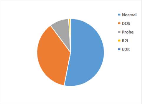
Fig.1. Class Distribution for the NSL-KDD Intrusion Dataset

It is easy to observe from Figure 1 that our NSL-KDD dataset suffers from severe imbalance. The R2L and U2R classes are under-represented, while Normal, DoS and Probe classes represent the majority of the instances. Unbalanced or skewed datasets is one of the major problems that face many researchers when using learning curves to predict the minor classes. In terms of detection accuracy, the detection rate for the minor classes is very poor or sometimes none [11].

This problem is very obvious when plotting the learning curve, where the accuracies for the minor class are very low or even zero at some given sample sizes. The training points are found to be very scattered, thereby making the fitting process hard or sometimes not possible.

• V.    Performance of Naïve Bayes Classifiers

In this section we describe the performance of Naïve Bayes classifiers with respect to individual classes in the NSL-KDD dataset. More precisely we describe for each class C in our dataset the accuracy of the classifier to correctly classify a record that belongs to the class C . Of course this accuracy depends on the size of training sample, i.e. the number of training examples, and also the popularity of the questioned class in these examples. We use the F-measure (described in Section III-B) to measure the accuracy of the classifier relative to every class.

To investigate the impact of the sample size on the performance of the classifier with respect to each class, we vary the sample size ε from 1% to 50% of the total dataset size and for every value of ε we perform the following procedure.

• 1)    For i = 1,2,…, 10 do steps 2 to 4.

• 2)    Draw a random sample S_i of size ε records from the dataset.

• 3)    Train a Naive Bayes classifier B i on S i .

• 4)    Using the remaining records in the dataset for testing, evaluate the accuracy of B i with respect to each class.

• 5)    For each class C evaluate the average accuracy of the 10 classifiers B 1 ,…, B 10 with respect to the class C and plot this average accuracy against the sample size ε.

The above experiment yields five plots where each one corresponds to one class C and describes the relation between the training sample size and the average accuracy (measured by the f-measure) of correctly detecting records of C . Figure 2 displays these plots together with an additional plot which displays the weighted average accuracy for all the classes. This procedure is implemented using the JAVA language along with WEKA library [37] as a data mining tool.

It is important to observe from Figure 2 that the classification performance for minority classes, i.e. R2L and U2R is very poor compared to other classes. This is because the minority class is relatively unlikely to appear in the training sample and therefore the classifier is unable to learn well to detect such a class. Note also that for all classes the small training samples exhibit bad and unstable performance due to the lack of enough examples that allow the classifier to detect the classes reliably.

• VI.    Constructing the learning curve

In the previous section, we described our experiments to evaluate the classifier performance given random training samples of variable sizes. In the following we aim to find an approximate relation between the training sample size and the classifier performance. More precisely we use curve fitting techniques to construct the learning curve of the classifiers, which establishes the required relation.

For the fitting process, we used two versions for the power law model. The first model is the two-parameter power law described in (5) while the second one is the shifted power law having 3 parameters. These two models are summarized in Table 1.

Table 1. Power-law Regression Models

Model Name	Formula
Power Law	a xα
Shifted Power Law	a (x - b)α

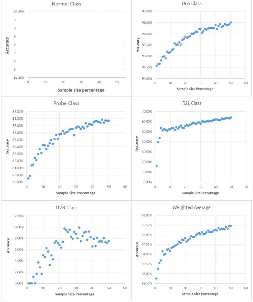
Fig.2. Performance of Naive-Bayes Classifier for Individual NSL-KDD Classes

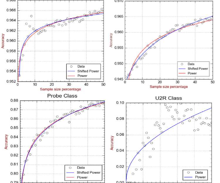
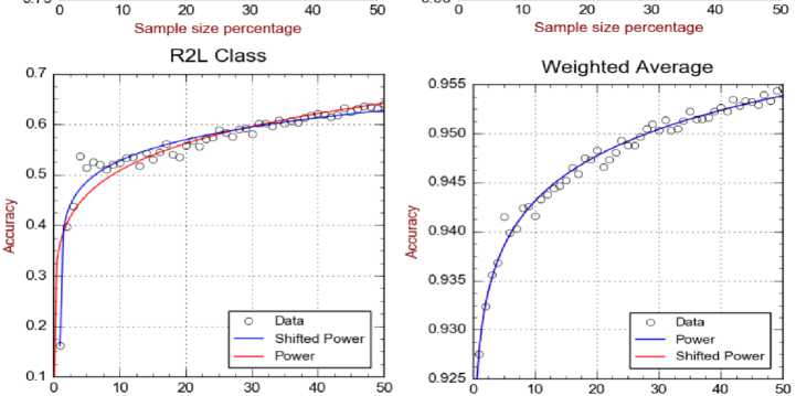
Based on the performance data that we demonstrated in Figure 2 we construct the learning curve for every class using the two non-linear regression models in Table 1. More precisely, we fitted 50% of the full-length dataset with respect to every class in our intrusion dataset. Figure 3 demonstrates the results of the curve fitting applied to every class in the dataset.

A first observation from Figure 3 is that the learning curve varies from one class to another. More precisely, the naïve Bayes classifier that learns from a given training sample has variant accuracies to recognize various classes. For example, using 10% of the dataset for training the classifier, it can recognize the Normal class with accuracy 0.962, while it recognizes the less common R2L class only with accuracy 0.5. Of course these variations are due to the different proportions of these classes in the training set. Majority classes, e.g. Normal and DoS, are learnt at a higher rate compared to minority classes, e.g. R2L and U2R. However, all curves share a monotonicity property that the accuracy improves when larger training samples are used.

Normal Class                                DoS Class

Sample size percentage

Sample size percentage

Fig.3. Learning Curves for the Classes of the NSL-KDD Dataset

It can be also seen from Figure 3 that the growth of the learning curve (with the training sample size) varies from one class to another. In particular, the accuracy for the classes Normal grows from 0.962 at sample size 10% to 0.966 at 50%, i.e. gaining only improvement of 0.004. However the accuracy for the minority class R2L grows from 0.5 at sample size 10% to 0.65 at 50%, i.e. gaining a larger improvement of 0.15. This is again due to the majority of the Normal class compared to R2L. In fact 10% of the training set is sufficient for the classifier to learn the majority class well such that more introduced examples do not much improve such learning. This situation is clearly different for the minority class R2L, where enlarging the training sample significantly improves the learning quality.

When the target class is a rare or minor, the task of obtaining a good accuracy estimate needs an excessive sample sizes. This is clear in the U2R class, where the number of records is very low in the given training samples. This causes the points of the data points to be very scattered (as seen in Figure 2), and therefore significantly lower the quality of the learning curve. In order to tackle the problem of the low detection rates for both R2L and U2R classes, we applied both sampling methods (Over-sampling and Under-sampling). However, results showed no improvement in the detection accuracy for both those classes.

Researchers in [38] showed that the problem of detecting U2R and R2L cannot be simply solved by resampling techniques since the problem is not directly related to the class imbalance. The unsatisfactory detection results were explained using a matrix plot, shown in Figure 4, which showed a clear overlap between these two attack classes. As a consequence of this overlapping, the decision boundaries of these two rare classes could not be generalized clearly by the learning algorithm. This shows that sometimes it is not worth the effort to collect more samples for a given class.

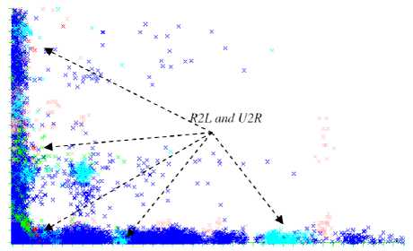
Fig.4. Class overlap problem for U2R and R2L [38]

Finally we remark that the weighted average learning curve is clearly impacted by the major classes and masks the poor quality of the classifier with respect to minority classes. This proves the importance for studying the learning curve for individual classes, instead of studying only the average learning curve.

• VII.    Fitting Performance (Goodness of Fit)

In the following we compare between the goodness of the two non-linear regression models listed in Table 1. In this comparison we use the following two measures.

• •    Residuals Standard Error (RSE) [39]: This error is evaluated as

RSE = (HEE ,                (7)

DF where SSE is the Sum of Squared Errors given by (6) and DF is the degree of freedom, defined as the number of dimensions in which a random vector might vary [40]. For nonlinear regression models, DF can be defined as a measure of optimism of the residual sum of squares (RSS) [41]. It is calculated as the number of data points minus the number of parameters for our model [34].

• •    R-squared [42]: It is a statistical measure known

also as the coefficient of determination. Similar to SSE and RSE, it measures how close the data is to the fitting regression curve. Precisely, it is defined as

R ² = 1

SSE

SST ^,

where SSE is the Sum of Squared Errors (6) and SST is the Total Sum of Squares which is the sum of squared deviations of the data measures y i from their mean ȳ , i.e.

SST = £ ( y, - y ) 2 . ⁽⁹⁾

Note that R2 quantifies the goodness of fitting the data relative to SST which quantifies the variability of the data itself from its mean. Note also that in contrast to RSE, the value of R2 increases when the regression is improved.

For the sake of comparison between the qualities of the two regression models in Table 1, we evaluated the RSE and R2 for all learning curves that we constructed in Section VI for individual classes in the intrusion dataset. The resulting values are shown in Tables 2 and 3.

It is clear from these tables that the shifted (3-parameters) power law outperforms the simple power law model in terms of both RSE and R-squared. This is explained by the fact that the shifted power-law has more parameters than the power-law making the former more flexible and hence yielding a curve that is closer to our data points. We remark that in the case of the U2R class the regression based on the shifted power law failed to converge due to the very low number of records of this class in all training samples, making the estimation of the three parameters of the model unstable.

• VIII.    Predection Performance

The technique of predicting the performance of a model at data beyond the available observations is known as extrapolation. Applying this technique to our problem allows us to use the learning curve that is constructed on a range of training sample sizes to predict the quality of the classifier when trained on larger samples. This curve can be also used to estimate the appropriate size of the training sample in order to reach some desired criteria, e.g. obtaining a certain accuracy of detecting a given attack class, or reaching a minimum value for the overall accuracy.

Table 2. The Fitting Performance of Power-Law Models in Terms of RSE

	Residual Standard Error Normal          DoS          Probe         R2L         U2R      Weighted Average
Power Law	0.001053	0.001349	0.00320	0.03561	0.0163	0.0007
Shifted Power Law	0.000941	0.000787	0.00299	0.01581	----	0.0007

Table 3. The Fitting Performance of Power-Law Models In Terms of R2

	R2 Normal DoS  Probe  R2L   U2R    Weighted Average
Power Law	0.82	0.94	0.97	0.79	0.67	0.98
Shifted Power Law	0.86	0.98	0.98	0.95	----	0.98

It should be noted that the fitting performance for a model might be deceptive. In other words a model might exhibit a high fitting performance but however a very poor predictive performance. This is known as the problem of ‘overfitting’. More precisely the model is said to be ‘overfitting’ when it significantly fits the training data but yields weak estimates when it is tested on new observations [4].

In order to evaluate the prediction performance of a fitting model, we use subsets of only a small portion, e.g. 10% of the dataset to construct a learning curve, based on the given model, and then examine the ability of the resulting curve to extrapolate larger samples, i.e. its ability to fit the actual accuracy of the classifier when it is trained on larger samples. More precisely we measure the absolute difference between the predicted accuracy at a large sample size using the curve and the real accuracy obtained by training the classifier on a sample of the same large size. The average difference (considering all large sample sizes) is called the prediction error for the model. The model that yields the less prediction error is the better.

In our experiments we restricted the construction of the learning curves to variant small portions of the dataset, specifically 10%, 20%, 50%, and in each case we evaluated the prediction error of the model for every class in the dataset using the aforementioned procedure. Table 4 demonstrates the results of this evaluation for the power-law model. We also applied the same evaluation method to the more flexible shifted power-law model for which the prediction errors are demonstrated in Table 5.

Table 4. The Prediction Errors of the Power-law Model

	Power Law
	Normal	DoS	Probe	R2L	U2R	Weighted Average
10%	0.007	0.005	0.004	1.44	0.28	0.0006
20%	0.003	0.0006	0.003	0.19	0.06	0.0005
50%	0.001	0.0008	0.003	0.05	0.03	0.0005

Table 5. The Prediction Error of Shifted Power-law Model

	Shifted Power Law Normal  DoS  Probe  R2L  U2R   Weighted Average
10%	0.001	0.004	0.019	---	0.03	0.0017
20%	0.008	0.001	0.005	---	0.03	0.0009
50%	0.003	0.001	0.005	---	0.01	0.0005

It can be seen from the above tables that the prediction power is generally improved as more samples are used for the fitting process. For instance the prediction error of the power-law with respect to the Normal class is 0.007

when only 10% of the dataset is used for constructing the learning curve, and this error drops to 0.001 when 50% of the dataset is used for that construction.

It is also important to observe that the power law model tends to outperform the shifted power law in terms of the prediction error. This is clear in the majority classes Normal, DoS, and Probe. However this observation does not hold for minority class U2R due to the instability of their learning.

• IX.    Conclusions

In this paper, we investigated the relation between the size of training set and the performance of an intrusion detection system working on NSL-KDD dataset. Our basic tool for this purpose is non-linear regression models. A model should be good in predicting performance as well as fitting performance. We compared two power law models and tested their fitting performance as well as their predicting performance. The curve fitting procedure was evaluated on each class in our intrusion dataset. It was shown that the number of instances for a given class greatly affects the fitting process. As expected, due to its flexibility, the three parameters shifted power law yields a better fit than its power law counterpart. However, it failed to fit the U2R class due to the very small number of records in this class.

We also investigated using the learning curve to predict the classifier performance when it is trained on large samples. For this purpose, we used only a small training portion of the dataset to construct a part-length learning curve by applying curve fitting using one of the two power-law models. The part-length curve is then extrapolated to a full-length curve and compared to real performance data at larger samples. This experiment was performed for random data portions of sizes 10%, 20%, 50% of the original dataset, and using the two power-law models. In every case, the average prediction error is evaluated for each class by averaging the absolute differences between the predicted accuracies on one hand, and the observed accuracy when the classifier is really trained on the large sizes on the other hand. These experiments were conducted using JAVA language along with the WEKA machine learning tool. We find that the prediction power generally increases as more samples are used for the fitting process. Our experiments reveal also that the power law model with fewer parameters outperforms the shifted power law in terms of predicting the classifier performance at larger sample sizes.

Our future work includes considering other fitting models and more intrusion datasets. Also, we plan to study more classifiers other than the probabilistic Naive Bayes.