Estimating the Video Registration Using Image Motions

Published Online July 2012 in MECS

The purpose of this paper is to outline a technique for finding the registration between two frames from a sequence of video that corresponds to the camera motion that also provides a means of detecting, and approximately segmenting, the moving objects within that scene. The approach taken is to split the image up into a series of blocks, and run a search comparing different registration parameters to find the transform that most effectively maps the motion of the scene background by means of grouping.

A sequence of video generally involves two main unknowns: the movement of the camera, and the form and motion of the moving objects in the scene. This can involve many different motions, all of which must be detected and calculated separately, which is a very difficult task.

Image registration is the process of matching a pair of similar images in terms of the rotation, translation, scale and shear required to make those images correctly align. The particular focus of this paper is the application of this on two frames from a video sequence to describe image motion. Applications include automated image and video inpainting for special effects in the film industry, use with mobile security systems, and vision systems for autonomous agents.

For images that do not contain moving objects, the process of extracting information about the movement of the camera for the scene is relatively straightforward – by using an affine transformation model it is simply a matter of finding transformation parameters (rotation and translation) that match the two images using a simple error metric like sum of squares difference. However, once moving objects are introduced to the scene, the registration process becomes more complicated. For a situation where the motion of the camera is unknown, and the location of any moving objects is unknown, a registration algorithm has a significant amount of information that it needs to infer.

Different sections of the images will have different motions (for example the background moving in one direction due to camera motion, while a person walking through the scene moves in a different direction). These areas of separate motion need to be identified and the magnitude and direction of the motion needs to be independently calculated.

This paper looks at an approach to this problem using a block-based technique for the registration. This enables differentiation between the dominant object in the scene (assumed to be the background) and other objects, which move relative to the dominant object. This provides information on the motion of the camera filming the scene.

• II.    METHOD

  • 2.1    Affine Registration

The technique used for registration in this paper is parametric affine registration. We currently restrict the algorithm from full affine to a three-parameter model, using rotation and x- and y- translation. The decision to ignore shear and scale considers that the effect of these between adjacent frames in standard video is likely to be minimal, and the block-based approach should allow for this to be detected without explicitly searching for it. Though it may have some impact on accuracy, the gain in efficiency obtained by ignoring scale and shear is significant.

The three-parameter affine transformation model for mapping the registration of a single pixel between two images ( I 0 and I 1 ) is as follows

ƒx0,y0= x1y1 = cos(θ) sin(θ)-sin(θ) cos(θ) + x0y0 + txty where x0y0 is the position of a pixel in the original image I0 and x1y1 is the position of the corresponding pixel in the second image, I1.

The rotation is conducted about the point (0 , 0) on the image (the top left corner), so for a different centre of rotation the image must be offset. The values t x and t y are the x- and y-translations respectively.

The registration itself is a minimisation problem: identifying values for t x , t y , and θ that minimise an error value between image I 1 and the transformed I 0 . The error used for this paper is the sum-of-squares difference between the RGB colour values of each pixel over the image or image section:

ɛ =Σ ( ɪ 0 (x i ,y j )-ɪ 1 ( ϝ (x i , y j ))) ²

As algorithmic efficiency is a major concern, the use of a gradient descent algorithm to optimise the search was investigated. For this application, however, gradient descent is not ideal the frequent occurrence of local minima throughout the search space, a high susceptibility to noise, and an inability to effectively process areas of low colour differential severely hamper its effectiveness.

• 2.2    The Integration Approach

Attempting to match a transform to the entirety of an image is impractical for a registration technique on video containing moving objects, as different parts of the image will be moving different amounts. Therefore, it makes sense to acknowledge that there will be objects, and allow them to be excluded from the registration. Methods like optical flow can achieve this by mapping pixels individually, but individual pixels are highly susceptible to noise, which can in turn affect the registration.

If working over the entire image is too broad, and looking at individual pixels is too fine, then it is logical to try and find a sort of middle ground. By splitting the image up into a series of blocks and tracking these separately, errors caused by certain types of noise (most notably, the blurring that is a common result of video compression) can be minimised, and sections of the image containing moving objects can be eliminated from the registration problem.

There are two approaches to the block-based image registration. The first involves running the registration search algorithm for each block individually to calculate the best transform for each block. These results can then be correlated in the form of a three dimensional histogram, where the largest group corresponds to the transformation that describes the motion of the largest ‘object’, which can be taken to be the background.

This method is inherently slow, as the search space is fairly large. For this reason, an iterative search approach over a multi-resolution pyramid is employed. The algorithm is initially run at quarter-scale or smaller (depending on the size of the original image) with broad search parameters, then the results are aggregated and used to determine a much smaller search area, which is then applied to a half-scale image. The search parameters are then refined again, before finally being applied to the original full-scale image.

Susceptibility to noise and difficulty distinguishing large areas of colour lead to a proportion of blocks returning incorrect results for the registration. For this reason, at each stage of the refinement the overall best result is used as the base for the next iteration of the registration for each block.

The second method is considerably faster, but also introduces a much greater potential for error. It involves picking a block at random and running the affine search over that sole block to find the transformation that fits that block to the next image. That transformation is then applied to all the blocks and thresholding is used to identify which blocks agree with the transform, which in turn gives the approximate area of the object whose movement is mapped by the transform.

In theory, this algorithm appears to solve the problem that is the target of this paper: identifying and tracking each individual object in the scene. In practice, however, this is unachievable. Firstly, there are the blocks that contain parts of more than one object; these will seldom match the transform of any object, so will not be grouped correctly. Similarly, blocks that is resampled to by the algorithm and that exist in areas of solid colour (i.e. have no distinguishing features/colours) will likely not track correctly, which would also interfere with the results.

Figure 1 show the chosen transformations for a registration search run over an image pair using 20x20 blocks. Only a single search is run on the full-scale image, to demonstrate the registration process without the corrective measures that are used in the iterative coarse-to-fine search. The number of blocks that produce conflicting registrations demonstrates the high occurrence of local minima over the search, and thus the necessity of the corrective groupings used in the iterative search.

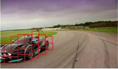
Fig. 1. This shows the detected motion paths of blocks across the image after one iteration of the affine search on the full-scale image. (See Figure 3 for the images used in this registration). The necessity of an iterative search approach is shown by the number of apparently random motion paths that are produced.

• 2.3    Extracting Object Information

The extraction of object information is based on the premise that most of the image is background, which moves according to the motion of the camera, with certain sections of the image not conforming to this motion – those sections belonging to independently moving objects.

For the purpose of comparison, a second method based on a difference algorithm applied postregistration is used. The algorithm uses the existing block structure to reduce the impact of noise on the results. Each block is marked as belonging to an independently moving object if sufficient pixels within the block are significantly different. The level of difference that is taken as significant is determined by an adjustable threshold, which requires changes depending on the level of contrast Fig. 2.Example of detection of a moving object using the block-based method. The image was first registered to a second image, then the block information was used to highlight moving objects within the scene. The blocks shown on the image indicate the detected object area between background and foreground in the samples.

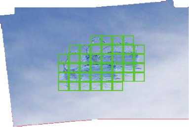
Fig. 2.Example of detection of a moving object using the blockbased method.

The image was first registered to a second image, and then the block information was used to highlight moving objects within the scene. The blocks shown on the image indicate the detected object area.

The method using registration information to identify moving objects works well in a broader range of situations. While the difference algorithm is often slightly more effective in high contrast scenarios, it struggles with low contrast.

• III.    RELATED WORK

• 3.1    Multi Integration Mapping

There are many methods of affine registration; good overviews of the work in the area are offered by [1], [2]. A common application makes use of registration techniques for mapping medical imaging scans to assist in the detection of anomalies, however the types of deformation involved do not transfer to the area of camera motion effectively. Patch-tracking is one area within the scope of registration and object tracking that has been pursued, with two different interpretations of its meaning available. The patch-tracking algorithm put forward in [3] is focused on tracking an object, and requires prior knowledge about the form of that object, which is not particularly useful here. [4] Offers an entirely different patch-based algorithm, which uses patches similar to the blocks used in this paper to solve regression equations for image distortion. The results presented here are impressive; however it does not deal with the existence of moving objects in the scene.

Window-based algorithms offer a similar sort of idea under a different name, such as those described in [5], [6]. These algorithms are designed to identify the camera motion in scenes with moving objects, and make use of gradient descent to find both the global minimum and a secondary, local minimum that describes the camera motion – this is specifically targeting scenes that are not dominated by background.

In terms of a registration approach to object segmentation, [7] establishes an effective foundation for work in this area, but the motion results contain some sections of image unrelated to the objects. [8] Presents with a more complete example of this approach, which is very effective, but the results are still influenced by outliers in the sequence. [9] Also provides some work in this area, but the resulting object segmentation displayed in the paper is patchy and incomplete. Another approach to the problem, using a pixel-wise optical flow method for registering and segmenting an image into its components, is presented in [10]. It produces some impressive results, but due to its pixel-wise nature the layers of the image will not separate completely, with some pixels being assigned incorrectly.

By introducing extra blocks across the image that overlap but are offset from the main registration blocks before the final fine-search of the registration, a higher degree of accuracy can be achieved for the object tracking at a certain cost in terms of computing power. These extra blocks are registered in the same way as the original blocks, and the results are aggregated using the logical AND operator to produce a finer resolution for the tracking result – only areas that are marked as moving objects by all of the blocks that contain them are included in the tracking result. This can be seen as a basic form of image super-resolution.

Figure 3 shows both the basic approach and the multi-block approach (using three extra block sets over the image). The multi-block approach provides a segmentation that does not include as much non-object data, but it still loses small sections of the edge of the object.

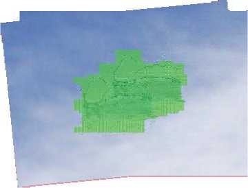
Fig. 3. The first image shows the object detection using the basic approach, with the detected object area shown by the registration blocks it is detected in.

The second image shows the multi-block approach, this time the detected area is shown as a grid to simplify the drawing algorithm. The images that the object detection is shown on is the mean image taken after registration (allowing the position of the object in both frames to be seen on the same picture).

• 3.2    Dynamic Textures Framework

• 3.3    Recovering the Spatial-Temporal Transformation from the Parameters of Dynamic Textures

Given a video sequence {I(t)} ^F t=1 , we model the temporal evolution of its intensities as the output of an LDS. The equations that model the sequence are given by

Z(t + 1) = AZ(t) + BV(t), (1)

I (t) = C ⁰ + C Z(t) + W(t). (2)

The parameters of this model can be classified into three types, namely, the appearance, dynamics, and noise parameters. The vector z (t) ε IRⁿ represents the hidden state of the system at time t. Its evolution is controlled by the dynamics matrix A ε IR^nxn and the input-to-state matrix B ε IR^nxq. These parameters are termed the dynamics parameters of the dynamic texture model. The parameter C ε IR^pxn maps the hidden state to the image and the vector C ⁰ ε IR^p is the temporal mean of the video sequence.

These parameters are called the appearance parameters of the dynamic texture model. The noise parameters are given by the zero-mean Gaussian processes v(t) ~ N (0,Q) and w(t) ~ N (0,R), which model the process noise and the measurement noise, respectively. The order of the system is given by n and p is the number of pixels in the image. The advantage of using this model is that it enables us to decouple the appearance parameters of the video sequence from the dynamics parameters. Thus, if one is interested in recovering appearance-based information from the video sequence, such as optical flow or, in our case, the spatial registration, then one only needs to deal with the appearance parameters. This allows us to recover the spatial registration independent of the temporal alignment of the sequence, as will be seen in the next section.

As motivated in the previous section, spatial registration can be recovered using a subset of the parameters of the LDS. In this section, we explore the relationship between the parameters of two video sequences that are spatially and temporally transformed versions of each other.

Let x = (x y) be the coordinates of a pixel in the image. We define Ci (x) to be the ith column of the C matrix reshaped as an image. Likewise, we define C0 (x) to be the mean of the video sequence reshaped as an image. With this notation, the dynamic texture model can be rewritten as

n

I(x,t) = ∑ z ⁱ(t)Cⁱ(x) + w(t),                             (3)

i=0

Where z⁰ (t) = 1. Therefore, under the dynamic texture model, a video sequence is interpreted as an affine combination of n basis images and the mean image. We call these n + 1 images {C ⁱ (x)}ⁿ i=0 the dynamic appearance images.

• 3.3.1    Synchronized Video Sequences

Let T : IR2 → IR2 be any spatial transformation relating the frames from each video, such as a 2D affine transformation or a homography. The relationship between two synchronized video sequence is then given by Ĭ (x,t) = I(T(x),t). Consider now the following LDSs, with the evolution of the hidden state as

z(t+1) = Az(t) + Bv(t),(4)

and the outputs defined as

n

I(x,t) = ∑zi(t)Ci(x) + w(t),(5)

i=0 n

Ĭ(x,t) = ∑ zi(t)Ci(T(x)) + W(t).(6)

i=0

We can see that Ĭ (x,t) = I(T(x),t). This shows that when a constant spatial transformation is applied to all the frames in a video sequence, the transformed video can be represented by an LDS that has the same A and B matrices as the original video. The main difference is that the dynamic appearance images {Cⁱ(x)}ⁿ i=0 are transformed by the same spatial transformation applied to the frames of the sequences, i.e., {Ĉⁱ(x) = Cⁱ (T(x))}ⁿ i=0 .

• 3.3.2    Unsynchronized Video Sequences

In this case, in addition to the spatial transformation, we now introduce a temporal lag between the two video sequences denoted by T . The relationship between two unsynchronized video sequence can be represented as Ĭ(x,t) = I(T(x),t + T). Now let us consider the following two systems, with the evolution of the hidden states given by (4), and the outputs defined as

n

I(x,t) = Σ z ⁱ(t)Cⁱ(x) + w(t),                             (7)

i =0 n

Ĭ(x,t) = Σ zi(t+T)Ci(T(x)) + W(t+T).                (8)

i=0

We now see that the above equations model two unsynchronized sequences. Thus, a video sequence that is a spatially and temporally transformed version of the original video sequence can be represented with an LDS with the same A and the same B as the original video sequences. However, in addition to the C matrix being modified by the spatial transformation, as in the synchronized case, we also have a different initial state. Instead of the video sequence starting at z (0), the initial state now is z ( Ƭ ). Nevertheless, if one wants to only recover the spatial transformation, the C matrices of the two LDSs are the only parameters that need to be compared.

Thus, given two video sequences, either synchronized or the unsynchronized, in order to recover the spatial registration, we only need to compare the C matrices. But this is under the assumption that both the A matrix and the state of the system z (t), modulo a temporal shift T i ε ℤ, for the two systems remain the same. The rationale behind this assumption is that since the video sequences are of the same scene, the evolution of the hidden states remains the same. More specifically, the objects in the scene undergo the same deformation; hence, they possess the same dynamics. However, if one learns the parameters of the LDSs from the data using existing methods, one encounter two problems. The first problem is that the A matrix is not the same for the different LDSs. Second, the C matrices that are recovered are only unique up to an invertible transformation. Hence, in order to perform the registration, we address these issues in the next section.

• 3.4    Recovering Transformation Parameters from The Dynamic Texture Model

• 3.4.1    Parameter Identification

• 3.4.2    Canonical Forms for Parameter Comparison

In the previous section, we have introduced the dynamic texture model and shown how the model parameters vary for video sequences taken at different viewpoints and time instances. In this section, we will show how the spatial transformation can be recovered using the parameters of the LDSs. In Section 3.4.1, we review the classical system identification algorithm for learning the parameters of an LDS and show that the recovered parameters are not unique. Since we would like to compare the parameters of different LDSs, our first task is to remove such ambiguities. This issue is addressed in Section 3.4.2. We then, in Section 3.4.3, show how we can enforce the dynamics of multiple video sequences to be the same. Finally, in Section 3.4.4, we propose an algorithm to recover the spatial and temporal transformation from the dynamic appearance images of two video sequences.

Given a video sequence {I(t)}^F t=1 , the first step is to identify the parameters of the LDS. There are several choices for the identification of such systems from the classical system identification literature, e.g., subspace identification methods such as N4SID [14]. The problem with such methods is that as the size of the output increases, these methods become computationally very expensive. Hence, traditionally, the method of identification for dynamic textures has been a suboptimal solution proposed in [12]. This method is essentially a Principal Component Analysis (PCA) decomposition of the video sequence. Given the video sequence {I(t)}^F t=1 the mean C⁰ = 1/F Σ^f t=1 I(t) is first calculated. The parameters of the system are then identified from the compact (rank-n) SVD of the mean subtracted data matrix as

[ I(1) - C0,..., I(F) – C0]=U(SV)T=CZ, (9)

where Z = [Z(1)... Z(F)]. Given Z, the parameter A is obtained as the least-square solution to the system of linear equation A[Z(1)... Z(F-1)] = [Z(2)... Z(F)].

It is well known that the factorization obtained from the SVD is unique up to an invertible transformation, i.e., the factors that are recovered are (CP-1, PZ), where P ε Irnxn is an arbitrary invertible matrix. Hence, the LDSs with (A, B, C) and (PAP-1, PB, CP-1) both generate the same output process. This fact does not pose a problem when dealing with a single video sequence. However, when one wants to compare the parameters identified from multiple sequences, each set of identified parameters could potentially be computed with respect to a different basis.

Since our goal is to compare the C matrices, to perform the registration we need to ensure that different C matrices are in the same basis. In order to address this issue, in the next section, we outline a method to account for the basis change. We propose to do this by using a canonical form and converting the parameters into the canonical form.

Given the parameters of an LDS (A, B, C), the family of parameters that generate the same output process is given by (PAP-1, PB, and CP-1). There are several approaches to removing the ambiguities from the system parameters. For instance, one can restrict the columns of the C matrix to be orthogonal. Exploiting this fact, one option to overcome the basis ambiguities is to project all the C matrices into the subspace spanned by one of the C matrices. In [11], Chan and Vasconcelos used such an approach where one sequence was chosen as the reference and the parameters of the other sequence were converted into the basis of the reference sequence. One drawback of such a method is that it requires a reference sequence. Choosing such a reference sequence might not always be feasible. An alternate approach from linear systems theory, to address the basis issue, is to use a canonical form. The advantage of such canonical forms is that the model parameters in the canonical forms have a specific structure. As a consequence, if the model parameters identified using the suboptimal approach is converted to the canonical form, the parameters are in the same basis. This removes the basis ambiguity induced in the suboptimal identification algorithm due to the SVD factorization. Also, using the canonical form does not require a reference sequence.

If one refers to the literature from linear systems theory, several canonical forms have been proposed for the model parameters of an LDS in the particular case of a single output system, i.e., p = 1. Although, in principle, any canonical form can be used to overcome the ambiguities, the fact that these LDSs model the temporal evolution of the intensities of pixels of a video sequence poses some constraints in the choice of the canonical form. For example, we do not want such forms to be complex. This would make it difficult to perform comparison between parameters of different systems. Also, even though, theoretically, all of the canonical forms are equivalent, in practice they differ in their numerical stability. Vidal and Ravichandran in [17] used a diagonal form for the A matrix. Since the equivalence class of parameters for A is PAP-1 , i.e., a similarity transformation, the diagonal form reduces to the diagonal matrix of eigenvalues of A. Thus, the resulting parameters in canonical form can be complex, since the eigenvalues of A can be complex. To overcome this, the Reachability Canonical Form (RCF) was used in [15]. The RCF is given by

B c = 0 0 0 … 1 ^T є R^nx1 ,                    (10)

where Aⁿ + a n-1 A^n-1 + ... +a 0 I = 0 is the characteristic polynomial of A and I n-1 is the identity matrix of size n-1. The problem with the RCF is that it uses the pair (A,B) to convert the system into canonical form. For most common applications of dynamic textures, such as registration and recognition, it is preferable to have a canonical form based on the parameters (A, C) because they model the appearance and the dynamics of the system. The matrix B, on the other hand, models the input noise and is not that critical to describe the appearance of the scene. Thus, a suitable candidate for the canonical form is the Observability Canonical Form (OCF) [16] given above by

However, the estimation of the transformation that converts a set of parameters to this canonical form is numerically unstable [16]. As a result, in the presence of noise, two dynamical systems that are similar can be mapped to dynamical systems in the canonical form that are fairly different.

In order to address this drawback, we propose to use a canonical form based on the Jordan real form. When A has 2q complex eigenvalues and n-2q real eigenvalues, the Jordan Canonical Form is given by

CC = 1 0 0 … 0  ϵ R1xn                    (11)

Cc = [ 1 0 1 0 … 1 1],                       (12)

where the eigenvalues of A are given by {б1 ± iw1 , б2 ± iw2,....,б q ± iw q ,λ1,...,λ n-2q ,}. It can be noted that the JCF is indeed equivalent to the RCF or the OCF, but in a different basis.

Given any general canonical form based on A and C, we now outline the steps to convert the identified parameters into the canonical form. Assume that we have the identified parameters (A,C). We now need to find an invertible matrix P such that (PAP-1 , TT CP-1) = (Ac,Cc), where the subscript c represents any canonical form. The vector T s IRP is an arbitrary vector chosen to convert the LDS (A,C) with p outputs to a canonical form, which is defined for only one output. In our experiments, we set T = [1 1....1]T so that all rows of C are weighted equally. The relation between the A matrix and its canonical form AC is a special form of the Sylvester equation:

A C P – PA = 0.

Vectorizing this equation, we can solve for P as vec(P) = null ( I ⊗ AC – AT ⊗ I ),             (14)

Where ⊗ represents the Kronecker product. Similarly, if we consider the equation between the C matrices, CCP = T T C, and vectorize it, we can solve for P by concatenating the two sets of equations as follows:

[ I ⊗ A C – AT ⊗ I I ⊗ CC ] vec(P)=[ 0 C]     (15)

Once we have solved this equation, we can convert the parameters into the canonical form using P. It should be noted that the JCF is unique only up to a permutation of the eigenvalues. However, if we select a predefined order to sort the eigenvalues, we obtain a unique JCF.

• 3.4.3    Joint Identification of Dynamic Textures

In the prior section, we have shown how to convert the identified parameters into the same basis so that we can compare the C matrices to recover the registration. However, comparing the C matrices to recover the spatial transformation is based on using the assumption that the A matrices for the two systems were the same. This assumption is valid as we observe the same scene, and since the hidden states z (t) captures the scene dynamics, they must evolve in the same way, irrespective of the viewpoint.

In this section, we propose a simple method to explicitly enforce the dynamics of multiple LDSs to be the same.

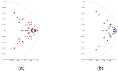
Fig. 4. Eigenvalues of the identified A matrices of two spatially and temporally transformed video sequences. The red crosses denote the eigenvalues for sequence 1 and the blue crosses denote the eigenvalues of sequence 2. (a) Separate identification. (b) Joint identification.

Consider M video sequences, each represented as I i ( t ) ε IR^Pi, t ε {1...F},i ε {1...M}. Let us introduce Ĭi ( t ) = I i (t) – C⁰ i for notational brevity. The traditional identification works by first forming the matrix Wi = [Ĭ i (1)...Ĭ i (F)], and then, calculating the singular value decomposition of Wi = U i S i V ^T i . The parameters of the LDS are identified as C i = U i (:,1 : n ) and Z i = S i (1 : n , 1 : n ) V i(:,1 : n ) ^T . In our approach, we instead stack all the videos to form a single W matrix and factorize it using the SVD as

W = Ĭ11… ĬF . . . ĬM1… ĬMF = USVT. (16)

Although this seems to be the intuitively obvious thing to do, we will now show that this is indeed the correct thing to do. If, for the sake of analysis, we ignore the noise terms, we obtain the state evolution as Z (t) = A^t Z 0 , where Z 0 is the initial state of the system. Now if we consider the temporal lag T i ε Z for the i th video sequences, then the evolution of the hidden state of the ith sequence is given by z i ( t ) = A^Ti z ( t ). Therefore, we can now decompose W using the SVD as follows:

W = C1AT1Z1 … C1AT1ZF CMATMZ1 CMATMZF

= C1AT1⋮CMATM (17)

From the above equation, we can estimate a single common state for all the sequences. Moreover, given Z, we estimate a common dynamics matrix for all the sequences. Now we can also recover C i from C up to the matrix A ^Ti. The problem is that T i is unknown, so we cannot directly compute C i from C. Now if we consider the equation for the ith video sequence, we can see that

[Ĭ(1)...Ĭi(F)] = C i A^Ti.[Z(1)...Z(F)] = C i A^Ti ( A^Ti)^-1[Z(Ti+1)...Z(F + T i )]. (18)

Thus, we see that the parameters we estimate are the original parameters of the system, but in a different basis. Therefore, by converting the parameters to the canonical form, we can remove the trailing ATi and recover the original parameters in their canonical form. The joint identification algorithm is outlined in Algorithm 1. Now, by construction, the A matrices of the multiple video sequences are the same. Hence, their eigenvalues are also the same. This can be seen in Fig. 4b.

Algorithm 1. Joint identification of video sequences

• 1    Given m video sequence { I i ( t ) ε IR^Pi } ^mi =1 , calculate the temporal mean of each sequence C⁰ i εIR^Pi Ĩ(t) =(t) -C^o i

• 2    Compute C;Z using the rank n singular value decomposition of the matrix

W = Ĩ11, … ,Ĩ1(F)⋮ĨM1, … ,ĨM(F) = USVT(19)

Z = SVT , C = U(20)

• 3    Compute

A =[z(2), . . . , z(F)][z(1), . . . , z(F – 1)] ε IRnxn.

• 4    Let Ci ε IRPixn be the matrix formed by rows V^1- 1     । 1   V-»-.

• 3 .4.4 Registering Using the Dynamic Texture Model

^j=i Pj - to ^j=i of C, and convert the pair (A,Ci) to Jordan canonical form.

Having identified a dynamic texture model for all video sequences with a common A and all C matrices with respect to the same basis, in the next section we describe a method to register multiple video sequences using the appearance parameters of the LDSs. Other applications of using the joint identification include recognition of dynamic textures, joint synthesis of videos, etc.

In this section, we propose an algorithm to recover the spatial transformation from the appearance parameters of the LDSs identified from the two video sequences. We need to compare this parameter between two LDSs, to recover the relative spatial alignment. In addition, the mean of the video sequence also contains information that can be exploited to recover the spatial alignment. In our paper, we term the mean image (C0) and the n columns of the C matrix as the dynamic appearance images. Let us consider two video sequences, I1 (x, t) and I2 (x, t), where x denotes the pixel coordinates andt =1, . . . , F. We assume that the video sequences are related by a Homography H and a temporal lag T , i.e.,I 1 (x, t) = I 2 (H(x), t + T). Once we recover the spatial alignment independent of the temporal lag between the video sequences, we temporally align the two sequences using a simple line search in the temporal direction, i.e.,T= argmin T ∑ t || I 1 (x, t) - I 2 (H(x), t +T)||²,T ε Z .

Our algorithm to spatially register the two video sequences I 1 (t) and I 2 (t) proceeds as follows: We calculate the mean images C⁰ 1 and C⁰ 2 , identify the system parameters (A, C 1 ) and (A, C 2 ) in the JCF, and convert every column of I C i into its image form. We use the notation C j to denote the ith column of the jth sequence represented as an image. We use a featurebased approach to spatially register the two sets of images {C⁰ 1, C¹ 1, ; . . . , Cⁿ 1 } and { C⁰ 2, C¹ 2, . . . , Cⁿ 2 }.

We extract SIFT features and aeature descriptor around every feature point in the two sets of n + 1 images. We match the features extracted from image Cⁱ 1 with those extracted from image Cⁱ 2 , where i ε {0, . . . , n}, i.e., the forward direction. We also match the features from Cⁱ 2 with those extracted from image Cⁱ 1 , where i ε{0, . . . , n}, i.e., the reverse direction. We retain only the matches that are consistent both in the forward direction and the reverse direction. We then concatenate the correspondences into the matrices X 1 ε IR^3xM and X 2 ε IR^3xM.

The corresponding columns of X 1 and X 2 are the location of the matched features in homogenous coordinates and M is the total number of matches from the n + 1 image pairs. We then need to recover a homography H such that X 2 ~ HX 1 . In order to recover the homography, we first run RANSAC and obtain the inliers from the matches. We then fit a homography using the nonlinear method outlined in [17]. Our registration algorithm is summarized in Algorithm 2.

Algorithm 2. Registration of video sequences

• 1    Given I 1 (t) and I 2 (t), calculate the parameters A, C⁰i , and C i .

• 2    Extract features and the descriptors from (Cⁱ j ),j = {1, 2}, i = 0, . . . , n.

• 3    Match features from Cⁱ 1 to Cⁱ 2 and also in the reverse direction. Retain the matches that are consistent across both directions and concatenate the feature point location from Cⁱ 1 into X 1 and its corresponding match into X 2

• 4    Recover the homography H using RANSAC such that X 2 ~ HX 1 .

• 5    Calculate temporal alignment T as T = arg min_T ∑_t ||I 1 (x, t) - I 2 (H(x), t+T)||².

• IV. EXPERIMENTAL RESULTS

• 4.1    Object Detection

• 4.2    Block Size

For this section, the algorithm developed in this paper, which builds object information as a consequence of the registration, is compared against a difference-based object detection method that is applied post-registration.

Figure 3 shows a pair of images that will be used for this test. The images have a moving object, and the camera is shifted and rotated between frames. Block size of 20 × 20 is used

The block sizes tested for the current incarnation of the algorithm is all square, mainly to keep things simple. The use of rectangular and other shaped blocks at this stage is unlikely to have any benefit.

The block sizes looked at for the test sequences (which measure 320 × 240 pixels) are as follows: 5 × 5 , 10 × 10 , 15 × 15 , 20 × 20 , 25 × 25 , 30 × 30 , and 40 × 40. The same sized block is applied to the reduced-scale images used for the initial coarse search conducted by the full-spread search algorithm (see Section II-B), as the minimum number of pixels required to produce accurate results does not change as the image gets smaller, since the size of a pixel remains constant. Figure 6 shows the mean sum of squares error for registration with different block sizes over three different image pairs.

When the algorithm is run with block sizes of 5 × 5 and 10 × 10, the number of pixels in each block is insufficient to accurately distinguish unique sections of the image and correctly map them in the registration. As a result, the registration at these block sizes is not sufficiently accurate to be useful. The object detection at this level is also not very effective, as essentially anywhere in the image with significant edges are picked up as deviating from the overall transform (since the transform is incorrect).

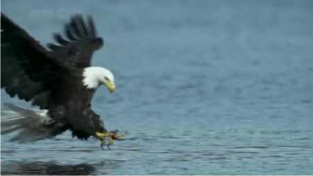
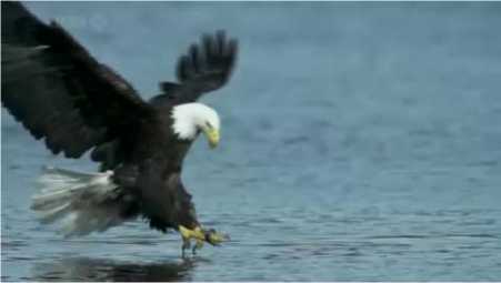
Fig. 5. Sample image pair for registration involving camera motion and an independently moving object.

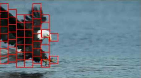
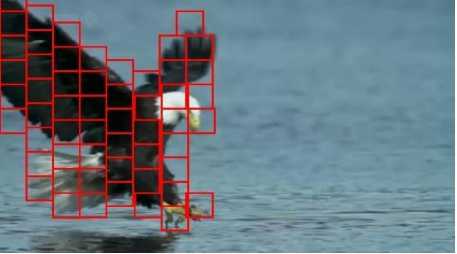
Fig. 6. Object detection using results of the block-based registration

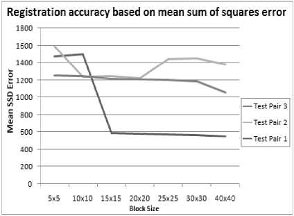
Fig. 7. Object detection using difference-based method

With a block-size of 15 × 15 to 25 × 25 the registration result remains the same for most image sequences, but in some cases 20 × 20 will give a more accurate result. In this case it can become a trade-off situation, since the smaller block size will give better object detail, but in most cases registration accuracy is the crucial element so a block size of 20 × 20 is best.

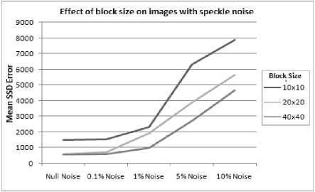
Fig. 8. Different amounts of speckle noise applied to sample images. This graph shows the accuracy of the registration using different block sizes for different noise levels. The difference in accuracy between the block sizes does not change very much over the changing noise levels, and beyond about 1% noise the accuracy is degraded too much to be useful.

• V. CONCLUSION

Dynamic texture of registering video sequences for recovering the spatial transformation independent of temporal transformation. Our result in the research shows that the methods reduce that number of frames at a time in one sequence. One needs to perform future extraction tracking and trajectory matching the multiset of F frames. In our case, we only need some extractions over for multi sets (n+1)*<< n images.