Estimation of NIIRS incorporating an automated relative edge response method

Today high resolution satellite images are being widely used in many applications and good quality images are of high demand from the users. Since interpretability is one of the most important quality metrics used in the case of satellite images, it is very important to have a system to assess the interpretability of a given image. The inference derived, helps us to understand the quality of the image as well as the performance of the imaging system. It helps us to make appropriate enhancements/corrections. Also, since images of different qualities will be having different applications, we will be able to categorize them based on the result obtained about the image. This was the motivation for the proposed work.

There are various factors viz. signal-to-noise ratio, ground sample distance, modular transfer function etc. which expresses the quality of satellite images. But these parameters can provide only a partial indication of image interpretability. Therefore, National imagery Interpretability Rating Scale (NIIRS) was proposed as an image quality metric in terms of interpretability. The proposed system uses NIIRS as the measure of quality.

• II.    Related Work

A lot of research is going on about the quality analysis of satellite images in the field of remote sensing. Many methods were proposed and new ideas are evolving for the quality analysis of the satellite images.

The metric that we discuss here does not exactly depend on the visual quality of the image. But both objective as well as subjective might be considered for Image Quality Assessment. In [1] Subjective versus Objective Picture Quality Assessment is discussed in detail. The calculation of NIIRS is explained in detail in [2]. NIIRS values are assessed by human operators for different high resolution images. This value is validated with that obtained using the image analysis method.

Edge detection is a vital phase in the proposed work. Study of various edge detection methods is done in [3] and [4]. [3] Discussed the edge detection techniques which could serve for the meaningful segmentation of an x-ray image. The main objective of the edge detection algorithms explained in [4] is to produce a line and to extract important features and reduce the amount of data in the image. Comparison of various edge detectors is carried out in [5] and [6]. [5] Compares the operators such as Canny, Sobel, Laplacian of Gaussian, Robert’s and Prewitt by the manner of checking Peak signal to Noise Ratio (PSNR) and Mean Squared Error (MSE) of resultant image. In [6] apart from the comparison of the traditional operators and methods, a new nature inspired algorithm, which can detect more number of edges is proposed.

[7], [8], [9] and [10] discussed edge profiling in different scenarios. In [7] text recognition is performed based on the edge profile. Also it used a set of heuristic rules to eliminate the non-text areas. At the same time [8] introduced a new method to recognize objects at any rotation using clusters that represent edge profiles. High-quality images can be recaptured from a liquid crystal display (LCD) monitor screen with relative ease using a digital camera. An Image Recapture Detection Algorithm based on Learning Dictionaries of Edge Profiles is introduced in [9] as a solution to this recent issue. Two sets of dictionaries are trained using the K-singular value decomposition approach from the line spread profiles of selected edges from single captured and recaptured images.  Finally an SVM  classifier is  used for categorization of query images. Similar dictionary of edge profiles is used in [10] for the identification of image acquisition chains. The processing chain of a query image is identified by feature matching using the maximum inner product criteria.

In [11] various image quality parameters such as Modulation Transfer Function (MTF), Ground Resolved Distance (GRD) and NIIRS are measured from the satellite images. [12] Demonstrates the effect of image compression on the ground sampling distance and relative edge response, which are the major factors affecting NIIRS rating.

Morphological operations play a vital role in the edge extraction phase of the proposed work. In [13] an ancient prominent fast algorithm for performing erosion and dilation is introduced which is independent of the structuring function size and hence suitable for signals and images that have large and slowly varying segments. An application of the morphological operations, detection of breast cancer is discussed in [14]. At the preprocessing stage, adaptive median filter is applied and followed by adaptive thresholding method at the segmentation process. The final stage uses morphological operations.

• III.    Proposed Work

Five quality metrics which express the interpretability partially are combined together to get the NIIRS value. These parameters include Ground Sample Distance (GSD), Noise Gain (G), Height Overshoot (H), Signal-to-Noise Ratio (SNR) and Relative Edge Response (RER). The final NIIRS level decides the characteristics of the image. For example, an image with NIIRS level 3 distinguishes between natural forest and orchards. Similarly from an image with NIIRS level 4, it is possible to identify farm buildings as barns, silos or residences and that with the level 5 identifies individual rail wagons by type (e.g. flat, box, tank). NIIRS is calculated using the equation in (1) which is known as General Image Quality Equation (GIQE). The GIQE focuses on three main attributes: scale, indicated using GSD; sharpness, measured using RER; and the signal-to-noise ratio.

The proposed system uses Relative Edge Response (RER) as a vital parameter for the estimation of NIIRS value. Hence all the prominent edges are extracted and considered for the finalization of RER of the image. Median filters of contrary neighborhood size are applied for the extraction of pure horizontal and vertical edges separately. Gradient and morphological operators applied in appropriate combination yields the detection of horizontally and vertically slanted edges. Proposed work made use of connected component analysis in order to limit the number of extracted edges. After the phase of edge extraction, the edge profiling is done by plotting the intensity values in the direction of variation of the same. RER is calculated as the slope of the edge profile that is plotted. Later NIIRS value is estimated by incorporating other parameters.

NIIRS = 10.251 - a log10 GSD + b log10 RER - (0.656 * H) - (0.344 * G / SNR)

In the above equation, a= 3.16, b=2.817, if RER < 0.9 and a=3.32, b= 1.559, if RER > 0.9

In remote sensing, Ground Sample Distance is the distance between pixel centers measured on the ground. In other words we can define GSD as the real distance (in meters) represented by a unit pixel of the satellite image. Signal to Noise Ratio gives a physical measure of the sensitivity of the imaging system. SNR value is calculated as the ratio of the mean of the image to the standard deviation. Height Overshoot (H) and Noise Gain (G) parameters are relevant when image restoration procedures are applied to the image. The increase in the overall noise of the image, as a result of restoration, is indicated by G. Relative Edge Response (RER) is the critical parameter in deriving the NIIRS value. RER evaluates how well an edge separates two different regions.

Being one of the prominent deciding parameters of the NIIRS value, accurate assessment of RER is very critical. The objective is to develop an automated system that calculates the RER value of a given image which will contribute for the computation of the NIIRS value. The prominent edges are extracted using a unique combination of filters and morphological operators. Connected component analysis also plays a key role in this part.

In this section we discuss the proposed framework in detail. Fig.1 illustrates the architecture of the proposed system. The initial step is the extraction of prominent edges from the input satellite image. It is followed by the profiling and computation of RER of horizontal and vertical edges separately. RERx and RERy represents the relative edge response of horizontal and vertical edges respectively. Net RER value is computed from RERx and RERy. Proposed method involves three phases viz. Edge extraction, Profiling of the extracted edges and Computation of RER. These three phases are explained in detail in the following sections.

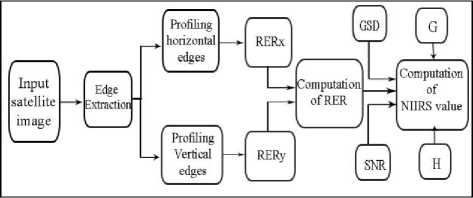
Fig. 1. Architecture diagram of the proposed work

• A.    Edge Extraction

Edge response (ER) is a measure of how well an imaging system is able to reproduce sharp edges in a scene. Relative Edge Response (RER) is defined as a geometric mean of normalized edge response differences measured in two directions of image pixels at points distanced from the edge by -0.5 and 0.5 ground sample distance. In an image there may exist edges which distinguish two regions well and which separate vaguely. That is, edges with different RER values can be present in the same image and all of them are to be considered to judge the overall RER of the image. Hence, the first step is to extract the edges. The architecture diagram of edge extraction is provided in Fig.2. Since RER involves the evaluation of edges with varying intensity values, edges are to be categorized as pure horizontal, pure vertical, horizontally slanted and vertically slanted edges based on the possibilities of these variations. In Fig.3 the variation of intensity values across three different types of edges is shown. From the figure, it can be seen that the variation occurs in vertical direction in the case of a horizontal edge and horizontal direction for a vertical edge. For a pure horizontal edge (Fig.3 (a)), the horizontal variation is zero. Similarly a pure vertical edge (Fig.3 (b)) has no vertical variation of intensity values. But the intensity

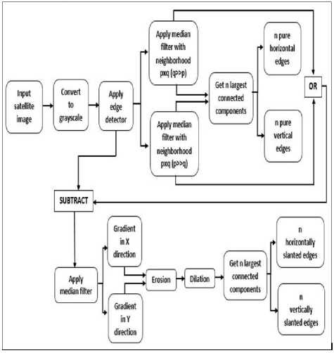
Fig. 2. Architecture diagram of edge extraction values vary in both directions across a slanted edge (Fig.3 (c)). So the ultimate objective of this phase is to extract horizontal, vertical and slanted edges separately.

We use Sobel edge detector in our method which gives an output of all the sharp edges being extracted, as shown in Fig.4 (b). It is evident that the edge detector gives all kinds of edges, many of which do not contribute to the calculation of RER. So the next step is to detect and extract the prominent edges that contribute to RER evaluation. In order to extract all the edges which are purely horizontal, a median filter with neighborhood pxq where q>>p is applied on the image that we got in the previous step (Fig.4 (b)). Similarly a median filter with neighborhood pxq where p>>q is applied on Fig.4 (b) to get all the pure vertical edges extracted. The extracted horizontal and vertical edges are shown in Fig.5 (a) and (b) respectively. Later connected component analysis is incorporated, if it is necessary to limit the number of edges to a particular number. Considering the size of the connected component to be an edge prominence metric, ranking the connected components in the order of their size and retrieving the first ‘n’ of them will give n prominent pure horizontal / vertical edges.

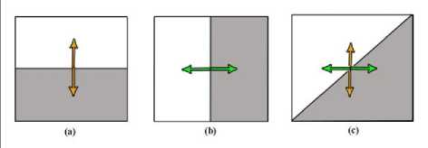
Fig. 3. Variation of intensity values across (a) pure horizontal edge (b) pure vertical edge (c) slanted edge

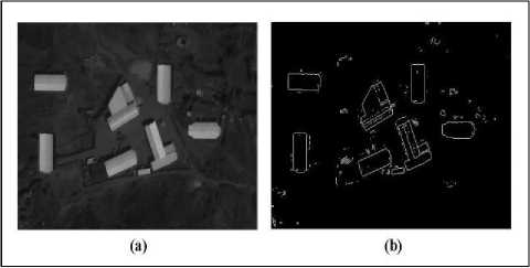
Fig. 4. (a) Input satellite image (b) Result of applying Sobel edge detector on the input satellite image

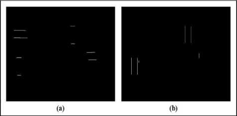
Fig. 5 (a) Extracted pure horizontal edges from Fig.4 (a) (b) Extracted pure vertical edges from Fig.4 (a)

The slanted edges that contribute for the decision of RER value are contained in the image that is just obtained

(Fig.6 (b)). With the objective of extracting them out as horizontally and vertically slanted, gradient operation is performed. It is good if a median filter is applied before going for the gradient operation, so that the unwanted insignificant edges which appear to be salt n pepper noise get removed.

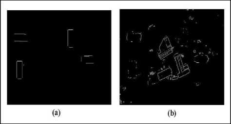
Fig. 6 (a) Union of pure horizontal and pure vertical edges (b) Result obtained on subtracting Fig.6 (a) from Fig.4 (b)

Equations (2) and (3) explains the gradient operation done on each pixel I(x, y) in X and Y directions respectively. Gradient operation performed in X direction gives the image with discontinuous broken horizontal edges. It retains the vertical edges. Similarly gradient operation in Y direction retains the horizontal edges.

X gradientX, У) = I(X + 1, У) - I(X, У) (2)

Ygradient(x, У) = I(X, У + 1) - I(X, У) (3)

Fig.7 (a) and (b) illustrate the outcome on applying the equations (2) and (3) respectively over the image shown in Fig.6 (b). It is evident from Fig.7 (a) and (b) that X gradient creates breaks in horizontal edges and Y gradient creates breaks in vertical edges.

Next step is to incorporate morphological operations. In the images that we have obtained from the previous step, first erosion and then dilation are performed using structuring elements of appropriate size. Actually we execute the morphological operation ‘opening’ through this, so that each component in the image becomes distinct. As a final step of this phase, the number of vertically slanted and horizontally slanted edges are limited by extracting the first ‘n’ largest connected components as shown in Fig. 7 (c) and (d).

• B.    Edge profiling

After the first phase, we have all the prominent edges extracted and categorized separately as pure and slanted horizontal and vertical. The second phase of the proposed method is to profile these edges. Edge profiling is very important for the evaluation of RER. We can define edge profile as a plot of intensity values of pixels on both sides of an edge. Fig. 8 illustrates the steps involved in edge profiling.

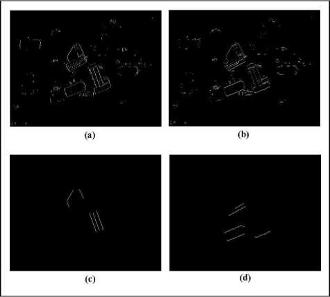
Fig. 7 (a) Result obtained on applying Xgradient on Fig. 6(b) (b) Result obtained on applying Ygradient on Fig. 6(b) (c) Extracted vertically slanted edges (d) Extracted horizontally slanted edges

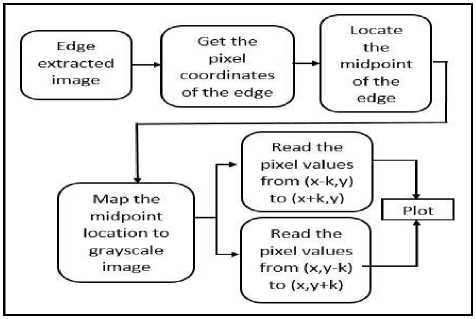
Fig. 8. Architecture diagram of edge profiling

It is necessary to map each edge obtained from the first phase to the intensity in order to do the profiling. A reference point is needed to do the mapping. In the proposed method, the central pixel of the edge which can be calculated using equation (4) is taken as the reference point. Fig.9 (b) illustrates how an edge shown in Fig.9 (a) gets extracted. In the calculation of the reference point, X coordinate is taken as the row number and Y coordinate represents the column number of an image.

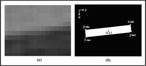
Fig. 9. (a) An edge in a grayscale image (b) Result of applying edge extraction on (a)

(xmax - xmin)

(x, y) = (xmin +                ,

ymin +

(ymax - ymin) 2

)

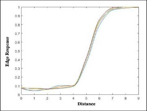
Fig. 11 (a) Plots of the set of pixels shown in Fig.10 against intensity value

After mapping the reference point on to the grayscale image, a fixed number of pixels say ‘k’ are chosen on both sides of the edge and their intensity values are plotted. Edge profiling can be defined as the plotting of intensity values of pixels that lie on a line which pass though the reference point by dividing the edge. In order to increase the accuracy of the plot, we choose two more lines of pixels from both the sides of the reference point to plot. The five plots are standardized to give a single final edge profile.

The selection of pixels to be plotted in the case of a horizontal edge is illustrated in Fig.10 It can be seen that (x,y) is the reference point and the line connecting pixels at (x-5,y) and (x+5,y) is considered as the reference line (indicated by red color). In the proposed method standardization is done by taking the average of the five plots as shown in Fig. 11 (a) and (b).

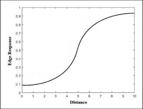
Fig. 11. (b) Normalized plot of (a)

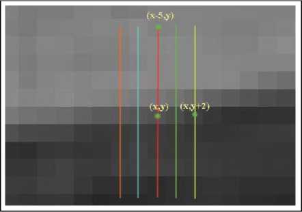
Fig. 10. Pixels to be considered for the calculation of RER

• C.    Computation of RER

As it was mentioned in the previous section, once the edge profile of an edge is estimated, it is possible to calculate the RER of that edge from it. Fig.12 explains how it is done. We can see that the edge response has been normalized by dividing by the largest intensity value of the image, so that it ranges from 0 to 1. Centre of the X axis say ‘c’ is taken as the centroid pixel of the edge and RER, which can be also called as the slop of the edge response is calculated as the difference between the edge responses at positions c+h and c-h. In Fig.12 the value of c is 5 and h is taken as 1.

The next objective is to calculate RER for a whole given image. For that, RER of all the ‘n’ pure horizontal edges are calculated by considering the variation in vertical direction alone. Subsequently, the average of these ‘n’ RER values is calculated, say RERx. Similarly RERy is calculated as the average of RER values of all the pure vertical edges, considering the variation in horizontal direction alone.

There are two ways of dealing with slanted edges. The first way is to club both horizontally and vertically slanted edges together as slanted edges and calculate RER for each of them as the mean of RER values obtained while considering the variation in both horizontal and vertical directions separately. After that the average of the RER values of these slanted edges is calculated as RERxy. Later RER of the whole image is estimated by finding the arithmetic mean, as shown in equation (5).

RERimage =

(RERx + RERy + RERxy)

The alternative method is to club pure and slanted horizontal edges together as horizontal edges and RERx is calculated as explained in the previous step by considering only the vertical variation. Similarly RERy is calculated after clubbing pure and slanted vertical edges. Finally RER of the given image is calculated by finding the geometric mean, as shown in equation (6).

RERimage = RERx * RERy (6)

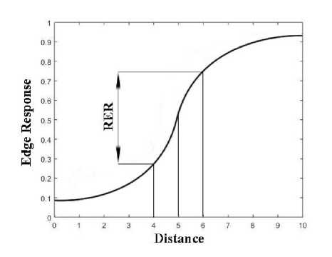
Fig. 12. Calculation of RER

• IV.    Gui Description

  The algorithm was implemented in MATLAB 2014b on Windows 7 with 2GHz CPU and 8GB memory. In the same satellite image itself, different edges gave different RER values. The algorithm could conclude the final RER of the image by considering the contribution of all the edges.

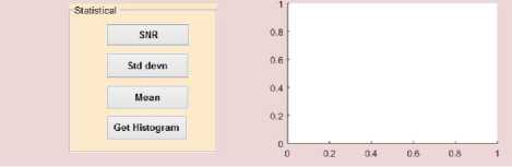
We provided two options to calculate the RER value of an image. The first one is fully automated in which the user’s job is just to load the image. The system calculates the RER using the method explained so far and reads the other parameters from the metafile of the image. The other option for the users is that they can select the edge from the image manually so that the RER of that particular edge will be given as the input parameter to calculate the final NIIRS value.

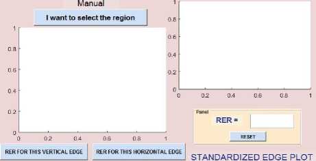
Fig.13 shows the initial page with which the system invites the user to it. The two options described above are provided as separate buttons. If the user clicks on the automated button, he/she will be redirected to the page shown in Fig.14 in which the calculation of RER and NIIRS is fully automated. The system gets redirected to the page shown in Fig.15 if the user opts to calculate RER manually.

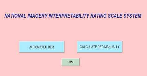
Fig. 13. Starting page of the system

(a)

(b)

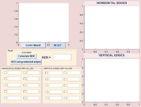
Fig. 14. (a) and (b) Page to which the system gets redirected when the button ‘AUTOMATED RER’ is clicked

selected edges)’ substitutes ‘Calculate RER’ and NIIRS respectively in this case.

(a)

(a)

(b)

Fig. 15. (a) and (b) Page to which the system gets redirected when the button ‘CALCULATE RER MANUALLY’ is clicked

(b)

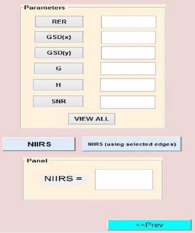
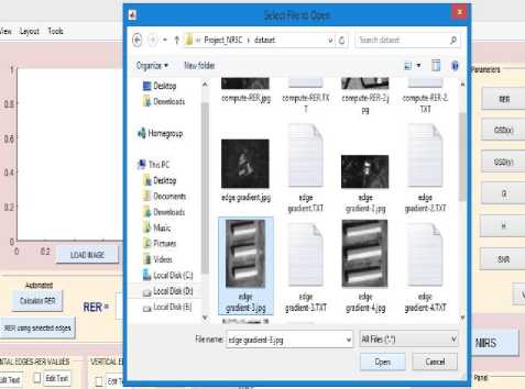
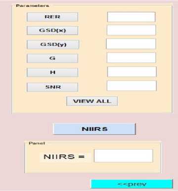
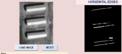
In the fully automated calculation of RER the user can chose the image for which RER and NIIRS values are to be calculated by clicking on the ‘LOAD IMAGE’ button as shown in Fig.16 (a). A click on the ‘Calculate RER’ button extracts the edges from the image and calculates RER using the proposed method discussed in the previous section. The edges used for the calculation are also displayed on the screen along with the RER value. Once the RER is calculated user can go for the estimation of NIIRS value. When the ‘NIIRS’ button is clicked, other parameters such as GSD are read from the metafile of the loaded image and final NIIRS value gets displayed on the screen. Fig. 16 (b) and (c) show the state of the system after the ‘NIIRS’ button is clicked.

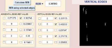
In the automated RER calculation itself another provision is added that the user can select those edges with their RER values in a particular range for the final estimation of RER of the image. Fig.17 (a) and (b) illustrate an example for this in which only edges with their RER values greater than 0.3 are selected. The buttons ‘RER using selected edges’ and ‘NIIRS (using

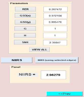
(c)

Fig. 16 (a) Loading the image (b) and (c) NIIRS of the image being calculated using the automated system

Automated

(b)

(a)

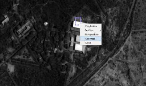
Fig. 18. (a) and (b) Edge being cropped by the user (b) Calculation of NIIRS of the image manually

(b)

Fig. 17. (a) and (b) Estimation of RER and NIIRS using selected edges

• V.    Results

The proposed method was tested on various satellite images through the implemented system and the results were tabulated and analyzed.

• A.    Dataset details

The following Table.1 gives the details of images used for NIIRS estimation. In certain cases, images of the same satellite will have different GSDs due to their difference in the viewing angles.

Table.1 Dataset Details

Image type	Acquisition date	GSD (m)
CARTOSAT-2 PAN	12-1-2008	1.0
CARTOSAT-2C PAN	12-1-2017	0.69
CARTOSAT-2C PAN	20-1-2017	0.69

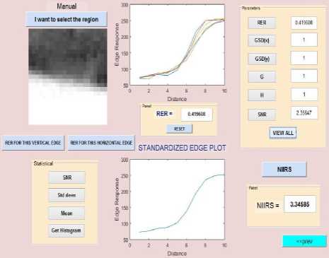
Fig.18 explains the estimation of RER and NIIRS using the manual intervention of the user. The cropping of the edge from the image on clicking the button ‘I want to select the region’ is given in Fig.18 (a). The selected horizontal / vertical edge alone will be considered for the calculation of RER of the image. Fig.18 (b) shows the estimation of NIIRS using the calculated RER and other parameters. It can be seen that the plot of the intensity values of the selected edge is also displayed on the screen.

(a)

• B.    Experimental results and analysis

The RER and NIIRS values obtained for certain Satellite images are given in Table.2 along with other parameters that are used in the estimation. Predicted NIIRS (PNIIRS) tabulated in the final column shows the NIIRS values obtained using GIQE image analysis through the proposed method. Since the final NIIRS value depends purely on the edges and the edge selection may change according to the methods used, the actual NIIRS value always lies in a range. The value that is obtained here is one of them in that particular range. Hence the name Predictive NIIRS.

Table.2 Estimation of rer and niirs

Image type	GSD (m)	RER	PNIIRS
CARTOSAT-2 PAN	1.0	0.29	3.41
CARTOSAT-2C PAN	0.69	0.53	4.69
CARTOSAT-2C PAN	0.69	0.42	4.40

It is evident from Table.2 that the final NIIRS level is much dependent on the Relative Edge Response. Also it can be inferred from Table.2 that the Predicted NIIRS has a direct relation with RER. But it varies inversely with GSD. This explains the reason for the reduction in quality of those images which are taken from greater height above sea level.

GSD is recorded in metadata for X and Y directions separately. Their geometric mean has been taken as the final GSD value for the calculations. SNR estimated for the entire image is used. Results obtained from automated and manual methods show similar patterns.

• VI.    Conclusion and Future Work

The NIIRS values estimated through GIQE followed same pattern and confirms with the published contemporary sensors imagery scales [15]. This confirms the values through GIQE represent actual interpretability of the image. Associating NIIRS rating with an image helps to establish a level of credibility for the IRS data products. An automated algorithm for NIIRS estimation by providing edge points is implemented in data products generation system.

The incorporation of General Purpose Graphical Processing Unit (GPGPU) processing in MATLAB to the implemented system is planned to improve the throughput .The RER estimation of several edges can be done in parallel and hence the net execution time of the system in the operational environment gets reduced. This is the proposed improvement plan for the existing system.

Acknowledgement

The authors would also like to thank the Department of Computer Science and Engineering, Amrita School of Engineering, Coimbatore for the support throughout the work.