Estimation of radio signal quality degradation by means of neural network and non-parametric regression model

The manufacturers of radio receivers and other radio equipment have to estimate the quality of the new product comparing to the existent equipment. Among other things the common listening comprehension of the perceived degradation with respect to the original (reference) audio signal has to be taken into consideration because humans with their own listening comprehension are supposed to be the main end-users of the designed equipment. Since any high-quality reliable subjective assessments are very expensive and time consuming it is strongly desired to have a tool for automatic perceptual evaluation of the audio quality degradation. This is a fundamental idea behind the PEAQ method, as specified in ITU-R BS.1387 recommendation [1]. According to this recommendation the PEAQ measurement method is applicable to the most types of audio signal processing equipment, both digital and analog. However, it is expected that many applications will focus on audio codecs. Test results obtained with the help of the PQevalAudio software, compliant with the basic model of PEAQ [2], disagree with the Mean Opinion Score (MOS) of the test persons. The Objective Difference Grade (ODG) of this software after appropriate linear rescaling is always significantly smaller than MOS. This implies that the PQevalAudio estimates the quality of the received (degraded) audio signal to be permanently lower than it seems to be for subjects from a test group. One of the obvious reasons is that the human requirements for audio files (signals) degraded by audio coding (recoding) are significantly higher than the requirements for files degraded by the entire radio transmitting-receiving process.

The output of the software is not only the final ODG value, but also 10-dimensional Model Output Variables (MOV's) combined using a neural network to give the ODG value [2]. Our goal is to create a new model having MOV’s as the input variables and to train it on the basis of our test group subjective estimations to be able to use the whole algorithm for automatic perceptual evaluation of transmitted through the radio channel audio quality degradation. We have chosen two different approaches for MOS approximation: neural network [3] and nonparametric regression model [4]. The performance of both algorithms on the test set is compared and the conclusions are presented in the corresponding section.

Alignment of Reference and Received Audio Signals. All test audio files are divided into two unequal parts. The smaller one consists of artificially simulated audio signals degraded by the additionally applied noise signals of different types, which sound more or less real comparing to the radio noise. The second part of the test audio material was obtained under conditions maximally close to the real situation – the reference short audio files were captured from various Internet radio stations with acceptable quality which were aired at the same time (with a small time delay) in our local area. Degraded audio files were captured from the corresponding radio stations in different conditions: inside the buildings and outside, in the driving car.

PQevalAudio software assumes two input audio signals (reference and degraded) to be time and gain aligned. Therefore, all the files are aligned even before the subjective assessment stage to be more accurate, when finding the dependency between MOS and MOV's.

Variable Delay Compensation. The reference and degraded files transmitted through the radio channel have not only a constant delay between each other, but also a variable delay changing through the entire audio signal. The constant delay is calculated as a maximum value of the cross-correlation function. The variable delay compensation is an increasingly complex process. Both reference and degraded stereo files are first converted into monaural ones and then divided into blocks of chosen length. For each pair of blocks the mean delay is found. This vector is then digitally filtered by the use of the normalized symmetric Hanning window. The result delay vector is then linearly interpolated for each sample and the final dynamic shift is performed by the cubic interpolation.

Usually the variable delay seems to have close to linear dependency from the time. However, sometimes due to the strong sudden noise or other distortions there are areas of the variable delay graph, where the curve seems to be almost randomly changing. In this case it is recommended to approximate linearly such «unreliable» areas using the left «trustful» data (see Fig. 1).

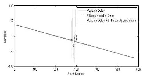
Fig. 1. Variable delay between reference and degraded files with and without approximation

In some specific cases the graph of the variable delay seems to change randomly. It is statistically estimated that in this case it is preferable to ignore the variable delay vector. The recognition of such case is automatically performed according to the acceptance threshold 0.1, i. e. the number of «reliable» data should not be less than 10 % of all block delays data. The smaller threshold would lead to the increasing of the average difference between files.

Gain Alignment. As a first step the reference and degraded stereo audio signals are converted into the monaural files. This should take into account, that the most of the receivers switch the audio to mono in the case of poor radio signal. Therefore, processing on the stereo signal may lead to a wrong gain calculation because of the reference and degraded files difference, caused even only by the switching to monaural signal, which can be quite pure itself.

The gain itself is calculated as the absolute value average of all samples of the monaural files. The sample values of the file yielding a higher gain are linearly reduced according to the gain difference. Then, the proportional normalization is applied for both files.

Subjective Assessments. Aligned files have to be estimated by the candidates from our test group. They should listen at first the reference and corresponding degraded audio files and then estimate the degradation of the second file with respect to the reference one. In our case each candidate has estimated 58 pairs of files, giving for every pair one value from the interval [0, 10] according to Table.

All pairs of files and appropriate MOS values are divided into two sets: training set used for model creation and the test set (10 pairs from 58). The data from the test set are not used for modeling to be honest in evaluating of approximation results.

Subjective estimation scale

Grade	Subjective impression
0	Program content is not/almost not understandable
2	Program content is in common understandable, irritative noise
4	Program content is mostly good understandable, especially when concentrating
6	Noise is (always) audible, also at the usual loudness
8	Reception distortion is audible when concentrating or at the high loudness
10	Reception distortion is inaudible even concentrating or at the high loudness

MSE ( C p ) =

<

s

1 z

⁵ i = 1

sn

y[i] -Z y[j ]ПФ j=1,        p=1

j * i

V V

sn ЕП ф j = 1, p = 1 j * i

x p ^[ i ^{] -} x p ^[ j ^] c p

( x p ^[ i ^] — x p ^[ j ^] )

V c p J

Neural Network Training. The modified approach for neural network training [5] by means of the genetic algorithm [6] is used. Genetic algorithms are global optimization stochastic algorithms which do not need the knowledge about the function and its derivatives. Only the values of the optimized function in the generated points are required for optimization [7; 8].

In our approach the genetic algorithm is applied two times within each iteration. Firstly it is used to optimize the weights of all neural nets in the current generation. The optimum in our case is the minimal value of the mean squared error (MSE) between the neural network output and the corresponding MOS values from a training set. Secondly the genetic algorithm is used to determine the new generation of the neural nets. In order to apply the optimization algorithm to a network structure its binary representation is used. The training is iterated until the stop conditions are satisfied or the break is performed manually.

Non-parametric regression model. Non-parametric kernel regression of a static object allows us to build a model of this object without any knowledge about the structure of the dependency between input (MOV’s) and output (MOS) variables. This model can be presented in the form of a next function:

y( x ) =

sn

Z y № i=1         p=1

sn

Z№R i = 1 p = 1      I

where Ф ( - ) is a kernel function; c p - smoothness

parameters, p = 1, n ; x [ i ], y [ i ] - input and output

variables from the training set, i = 1, 5 .

The kernel function should satisfy certain requirements [9] and in our case is chosen to be the following function:

^{Ф (} z )

f (3/4)(1 - z 2 ), [ 0, if\z\ >  1.

iTz\ ^ 1;

The only unknown parameters of the algorithm are smoothness parameters c_p which should be trained on the base of the available data, minimizing Mean Square Error (MSE):

To minimize this error one could use any optimization methods, especially stochastic methods aiming to find a global minimum, e. g. genetic algorithm. It is also possible to chose one single value of c and calculate all the   smoothness   parameters in the form of c = c (max x [i] - min x [i]). The parameter c should p            ip          ip be decreased from a fixed value (for instance, c = 0,5) with a fixed small step until the value of the MSE starts to increase. To get a better result the found values of cp should be adapted. We did a post-adaptation in our work manually; however, one could prefer a certain optimization method.

Experimental results. As it was previously mentioned, linearly mapped ODG value to the interval [0, 10] tends to be significantly smaller than MOS of the candidates from a test group (the MSE = 5,428).

The MSE of the difference between the output of the found neural network and MOS values calculated on the training data set is equal to MSE = 1,040 and calculated on the test data set is even smaller MSE = 0,971. The result approximation is at least much closer to the MOS, than linearly rescaled ODG software output.

Non-parametric kernel regression model on the same training data has achieved a little bit worse results MSE = 1,091 comparing to neural network. However, on the not-overlapping test data set the non-parametric model performed even better (MSE = 0,910) than our neural network. Moreover, it was found out that 6 out of the 10 sub-optimal smoothness parameters (according to 10-dimensional MOV’s) are much larger than the scale of the data in the corresponding dimensions. This means that these 6 input variables do not play any role in the nonparametric model and therefore could be omitted. We created a new non-parametric model on the base of the reduced data size (6 variables were ignored) with the same left smoothness parameters values (re-training of the parameters did not bring any improvement). The result model achieved MSE = 1,092 on the training set and MSE = 0,906 on the test set that is the smallest achieved error on this test set.

The results of both algorithms, rescaled ODG value and the perceptual estimations of the candidates (MOS) for 10 values from a test set are presented in Fig. 2. The closer the approximation to MOS is, the better the model is. Non-parametric regression presented on the graph uses only 4-dimensional input data.

Conclusion and Future Directions. Either the neural network or non-parametric regression model in combination with the PQevalAudio software can be used for the perceptual evaluation of the audio quality degradation, transmitted through the radio channel. The both approaches are obviously not as precise as the

subjective assessments. However, they could be used for the mean opinion score approximation.

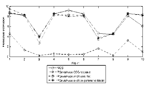
Fig. 2. The algorithms comparison

The non-parametric model has achieved slightly better results on the test set. The main advantage of this model is that we were able to exclude the insignificant features out of the model due to the huge values of the smoothness parameters. The input parameters left in the model are: «average block distortion», «distortion loudness», «noise-to-mask ratio» and «windowed modulation difference». The input parameters which were excluded from a model: «average modulation differences», «bandwidths of the reference and test signal», «harmonic structure of the error» and «relatively disturbed frames». The accuracy of the MOS approximation can be improved by the use of described algorithms trained on the considerably greater amount of data and estimated by a higher number of people.