Evaluation of Load Balancing Performance of Parallel Processing Linear Time-Delay Systems

Published Online May 2015 in MECS

Parallel computing is the dominant paradigm in system architecture of large complex systems. Different organisations like the Federal Bureau of Investigation (FBI) is using parallel computing techniques to develop and manage the Combined DNA Index System (CODIS) and National DNA Index System (NDIS) [1]. Simultaneous calculations are carried out in parallelcomputing systems, following the principle that big problems can be split into smaller ones and, then can be solved simultaneously. A busy computing unit may share some of its loads with a relatively idle computing unit, resulting in a significant increase in system performance and throughput. However, if these computing units are in a network, then information about the workload on the processing subunits is not instantly available to other subunits due to time-delay experienced during communication, which affects system performance adversely. Communication and synchronization among subsystems are typically some of the greatest challenges to performance in parallel computing [2].

Time-delay is one of the most significant issues for reliability in real-time control system. Time-delay systems are usually known as systems with deceased time, or systems of differential-difference equations, or systems of equations with deviation in argument. They are a constituent of infinite dimensional functional differential equations (FDEs) which are opposite of ordinary differential equations (ODEs) [3]. In clustered machine environment, additional communication delay is inevitable. This may lead to the system being unstable, uncontrollable or untraceable. The needs for observing time-delay in complex systems comes from the real requirement of system tracing, control and/or detection of system failure. In order to do so, it is often needed to redefine the parameters representing the states in a system with time delay. The difficulties concerning sensitivity along with robustness of the feedback system in regard to time delays has attracted much interest in academia and industries because of the effects of the time-delays on the performance of such systems. For a few systems, small delays result in destabilisation while many other systems are tolerant to small time delays [4]. In parallel computing, a significant amount of communication takes place among subsystems, therefore the subsystems experience time-delays during mutual communication that affects the system performance. The adverse effect of time-delay can be minimised by observing the states of time-delay systems and then utilising the information to model a linear time-delay system aimed at designing observers for all subsystems to minimise delays and increase stability.

This paper extends the work presented in [5], to evaluate load balancing performance of systems in the presence of liner time-delay. To do so, a linear time-delay system is modelled and simulated in SIMULINK to analyse the stability and performance of the system in performing load balancing operation. Stability is analysed in terms of oscillation in system responses. At the same time, performance is measured as speed of operation, i.e. how quickly the system can balance loads between subsystems. It is observed that the system responses oscillate more with higher gain in comparison to lower gain due to delays experienced by subsystems during communication. System gain is referred to as the reduction rate of waiting time (speed of operation) and value of system gain is constrained by delays experienced by the subsystems. During analysing the stability of the system, a linear control law is used instead of a saturated control law of real system. Because system responses oscillate more with linear control law therefore it is considerably easier to analyse the oscillatory behaviour of the system. After analysing system performance and stability, relationships among system gain, stability of the system performance and the delays experienced by the subsystems due to mutual communications are established. We have designed the observers for all subsystems of the parallel processing linear time delay system from the findings of these analyses. Observer of each subsystem estimates some necessary values for the subsystem to allow it to work independently without communicating with other subsystems thus minimising the effect of time-delay in the system performance. To evaluate the system performance the system with observers are modelled and simulated using SIMULINK.

The rest of the paper is organized as follows: Section II presents the background study and literature review on time-delay systems, observer design and load-balancing techniques. The parallel processing linear time-delay system is described, modelled, simulated, and results of the simulation are shown in Section III. In Section IV, observers are designed, system with observers is modelled, simulated and the result of the simulation is presented. Finally, a discussion on the results and concluding remarks are presented in Section V and VI respectively.

• II.    B ackground S tudy and L iterature R eview

• A.    Time-Delay Systems and Their Mathematical Models

Time-delay is an observable fact that occurs regularly in various systems, in different ways around us. A very familiar application where the delay arises is a live telecast on television. The video clip seen on TV differs in time from the actions take place in real time during live broadcast. Time-delay is encountered regularly in different control systems; either in the systems states or the control input [6]. Time-delay can be contributed as a source of instability in many systems. From a research perspective, the issue of delay is very important for performance and consistency of control systems. A considerable amount of research on performance analysis of time-delay systems has been performed in the last decade and researcher like [7]–[10] have contributed to stability investigation of time-delay systems. Robustness of time delay system is studied in [11]. Improved timedelay systems and stabilised controllers are suggested in [6], [12], [13]. A network-based controller for time-delay systems is studied in [14] and steadiness of networkbased control system is analysed in [15]. In [1], a linear time delay model was studied to see load balancing instabilities in parallel computing.

Time-delay system can be modelled in different ways. It can be described by the differential equation model, transfer function model, and others. A simple linear timedelay system can be represented as:

x (t) = ax (t) + bu (t) (1)

where a and b are constants, x(t) and u(t) are functions that change with time. Replacing x(t) by sin x ( t ) in (1), we find the following non-linear equation for the time delay system:

x(t) = a sin x(t) + b u(t) (2)

The equation can be rewritten for a time delay τ in following way with another constant c :

x (t) = ax (t) + bu (t) + cx (t — t) (3)

It is also possible to model a time-delay system using delay differential equation (DDE). In DDE, the derivative of an unknown function at a specific time is expressed with regard to the values of the function at earlier time. DDE is similar to ODE in mathematical treatment, but their evolution involves previous values of the state variables. Therefore it requires the knowledge of not only the present state, but also the state knowledge at a certain historical time for the solution of DDE. A general form of the time-delay differential equation for x ( t ) e R ^ is:

dx (t) = f (t, x (t), xt) dx

where x t = { x ( т ): t< t } represents the trajectory of the solution in the past.

Different types of DDE can be used to address delay of various natures. Equation (5) expresses a system with continuous delay:

For a system with discrete delay, the DDE takes the following form:

d- x ^(t ) = f ⁽ t , x ^(t ), ■•■, x ^(t - ^T m )) dx

for T i > т 2 > ^ > т _m >  0. DDE for a linear system with discrete delay takes following form:

dx (t ) = A 0 x ( t ) + A x (t - T j ) + ... + A m X (t - T m )   (7)

dx where Aq, A1,..., Am g Rwxn .

• B.    Control Systems and Observers

Control systems use sensors to determine and control the state of the variables/quantities like movement, heat circulation, temperature, stress, fluid pressure, etc. Sensors have some limitations [16] that may cause systems instability and problems like:

• •    Usually sensors are expensive that can raise the system cost significantly.

• •    Sensors itself and required wiring to incorporate in control system may reduce dependability and consistency of a control system.

• •    Occasionally, it is difficult for sensors to measure faint signal practically due to difficulty in accessing inconsiderate environment or relative movement between sensors and objects.

• •    Usually sensors bring about considerable errors such as cyclical errors, stochastic errors and limited responsiveness.

Internal states of many systems cannot be observed directly. This raises problems in feedback systems and consequently rules out the possibility of state feedback. A separate system, termed as an observer or an estimator that attempts to duplicate the values of the state vector, can be designed.

Observers are methods that merge with sensed quantities alongside the other information of the control system to generate control signals. Observers can be used to replace or as a supplement to the sensors in a control system. Observer generated control signals can be more precise, cheaper to generate, and more trustworthy than the control signals produced by sensors. Observers provide engineers an attractive option to accumulate new sensors or improve upon current ones [16]. A sample role of observer in a control system is shown in Fig. 1 and the general form of Luenberger observer is shown in Fig. 2.

• C.    Observers for Time-Delay Systems

System performance is affected by the delay introduced during system operation. An observer can be employed to observe the states of the system to address the time-delay problem. Different approaches like Kronecker canonical form, geometric, inversion approaches, algebraic, singular value decomposition, and generalised inverse techniques can be employed to design observer for systems with time-delay. Several varieties of state observer e.g., unknown input, disturbance decoupled, full-order, minimal-order, functional, etc. have been systematically investigated in [17]. Most frequently used observer systems are Luendberger observer, Kalman filter, and adaptive observer.

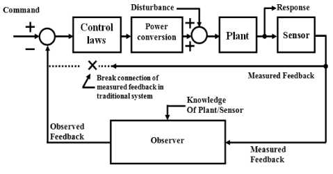
Fig. 1. Observer and Control System [16]

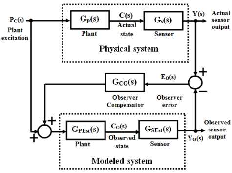
Fig. 2.General form of Luenberger Observer [16]

Kalman filter is often a recursive estimator for stochastic techniques, which usually consists of noise and processes with known parameters. It has a correction factor to insure stability of the observer through prediction and update. In predict step, it estimates current state variables and their vagueness. In update step, the current state variables are used to accurately enhance the estimation as it arrives at a new state estimate.

The ways of using a Kalman filter to design observer for time-delay systems were shown in [18]. The methodologies for designing robust observer for timedelay systems were described in [19], [20]. Time-delay system with memoryless state observer was presented in [21]. In [22], an observer for linear time-delay systems was designed using coordinate transformations. An observer for linear time-delay systems with unknown input was designed in [23]. Geometric design of observers for linear time-delay systems was proposed by Perdon and Anderlucci in [24]. Hou, Busawon, and Saif had discussed observer design techniques based on triangular form generated by injective map in [25]. Discontinuous observers for non-linear time-delay systems were designed in [26] and a neural observer was designed using coordinate transformation in [27]. Presently, network-based observer design is an emerging topic because of the constraint that all the required system components cannot be accommodated at same place in many systems. These components add further transmission delay by using network medium for communicating.

• D.    Load Balancing Techniques

In parallel computing, a group of processing units communicates and collaborates to solve big problems competently. Creating parallel programs requires first breaking the computation task into smaller chunks and distributing the chunks to the processors; this is called partitioning. The optimisation objective of partitioning is to stabilise the workload among processing units and to minimise the inter process communication needs. Some processors can become idle if the loads are not balanced properly among the processors; therefore efficiency of the parallel processing systems are dependent on the efficiency of the load balancing algorithms, i.e., how effectively the load balancing algorithm can evenly balance loads among the processors. Usually, a load balancing algorithm comprises of three stages – a) Information collection, b) Decision-Making and c) Data migration. The broad classification of load balancing were discussed in [28], shown in Fig. 3. This framework is suitable for explaining as well as classifying prevailing load balancing techniques, simplifying the task of finding an appropriate load balancing approach.

• III.    L inear T ime -D elay S ystem T o S tudy L oad B alancing P erformance

• A.    System Description

In many applications, in order to increase throughput and reliability, computer clusters are used instead of a single computer where a number of readily available computing nodes are available to facilitate parallel computing. In this paper, a computer cluster comprising of n nodes is considered which was first used in [1].

In the model, all the nodes can communicate with each other and at the very beginning of operation, all nodes are provided with equal work load. With the passage of time, the workloads on different processing units become uneven due to the varied processing capability of the processing units. To balance loads among nodes, each node in the cluster sends its load information qj (t) (queue length) to other nodes of the cluster. Due to timedelay node i obtains information sent by node j delayed by a certain period of time тij ; i.e., qj (t) is received as qj (t - тij) . After receiving information from all other nodes, each node locally calculates and determines the average amount of load using a simple

I nid q j ( t - т ij )

estimator — ■ j ¹ ■ -----—, where т ii = 0 . Then each node

n compares its own queue size against locally calculated queue size to make decision about task sharing. If the size of the queue of a node is greater than the average queue size then the node will send a portion of its tasks to other nodes. The scenario is shown in Fig. 4.

In the figure, the horizontal line indicates the average load predicted by processing unit 1 and the vertical bars represent loads for each node. As seen in Fig.4, node 1 has more load than the average estimated load of the network; therefore this node will decide to share its load with other nodes. In this example, node 3, 5, 6, and 8 are the nodes with fewer loads than average load in the network. Again, the sending tasks also add further delay in the course of its execution. As a result, node j receives tasks sent from node i with a time-delay of h_ij .

The load balancing procedure determines the frequency of performing load balancing operations. A smart load balancing algorithm should consider that each processing unit has delayed value of queue size and tasks send from one processing unit to other is received with a certain time delay.

• B.    Mathematical Model of the System

The mathematical model of the above system can be described as [1]:

dx ( t )                         ^{n       t} pi

~   = \ - Hi + u (t) -I pij    uj(t - hj )(8)

dt                        j=1  " tpj J ui(t ) = -Kiyi(t)

n

I x j ⁽ t ^{- т} ij )

У1(t) = xi(t)- — (10)

n where, n is the number of processing unit in the cluster; xi (t) is the estimated waiting time faced by a task placed into the queue of node i; Xi is the rate of increase of waiting time at node i and цi is the rate of reduction in waiting time at node i.

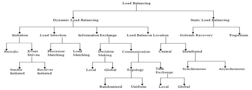
Fig. 3. Classification of Load Balancing Algorithms

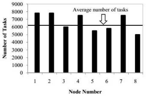
Fig. 4. General example of load balancing process

+ ^p 13 K 3 2 X 3 --⁽ X 1 ⁽ t - ^т 31 - ^h 13 ) + X 2 ^{( t - т} 32 ^{- h} 13 ))

Now if we consider the delay experienced by nodes during sharing load information as т ij — т and the delay to share tasks as h^ — 2т then the above equation takes following form:

X 1 = ^ 1 ^- H 1 ^- K 1

X 1 ^- g ⁽ X 1 + X 2 ^{( t - т)} + X 3 ⁽ t ^{- т))}

+ ^p 12 K 2

2 X 2 - 1( X 1 ( t - 3т) + X 3 ( t - 3т))

u_i ( t ) is the transmission rate of the tasks from processing unit i at time instance t to other processing units; p_iju_i ( t ) is the transmission rate of waiting time from node j to node i at time instance t where p >  0, p — 0 , and ij         jj

У nj^P^ij — 1; - P ij U i (t — h ij ) is the rate of transmission of the estimated waiting time from processing unit j by (to) processing unit i at time instance t where h_ij is the time delay for the load transfer from processing unit j to unit i and h_it — 0 ; and т ij is the time delay for communicating queue size from node j to node i.

In this paper, for simplicity, we have considered three computing nodes instead of n nodes generalised in the above equations. Hence, the equation for subsystem 1 in the cluster can be described as:

^{+ p} 13 K 3

2 X ₃ - 1 ( X ₁ ( t - 3т) + X ₂ (t - 3т))

= ^ 1 - Ц 1 ⁺ ”[ ^- K 1   ^p 12 K 2   ^p 13 K 3 ]

+ 1 [ 0   K 1   K 1 ]

^X 1 = ^ 1 ^- Ц 1 ^{+ u}1^(t ) ^{- p}11 ^u1^{(t - h} 11 ) ^{- p} 12 ^u 2 ^{( t - h} 12 )

^- P 13 ^u 3 ^{( t - h}13 )

= ^ 1 ^- И 1 ^{+ u} 1 ^{( t} ) ^- P 12 ^u 2 ^{( t - h} 12 ) ^- P 13 ^u 3 ^{( t - h} 13 )

= X 1 ^- Ц 1 ^- K 1

^X 1 ^- “ ^{( X} 1 ^{+ X} 2 ⁽ t ^{- т} 12 ) ^{+ X} 3 ⁽ t ^{- т} 13 ))

^{+ p} 12 ^K 2

2 X ₂

^-- ^{( X} 1 ⁽ t ^{- т} 21

^{- h} 12 ) ^{+ X} 3 ^{( t - т} 23 ^{- h} 12 ))

X 1

X ₂

X ₃

^--[ ^p 12 ^K 2 ^{+ p} 13 ^K 3   ^p 13 ^K 3   ^p 12 ^K 2 J

x ₁ - 3т

X 2 - 3т

X ₃ - 3т

Similarly, equations for subsystem 2 and 3 can be developed. After generalisation, the equations for all three subsystems can be written as:

X1 — X1 - Ц1 + a1 о X (t) + Q11X (t - т) + a13 X (t - 3т)(11)

X2 — ^2 - ^2 + a2,0X(t) + a2,1X(t - т) + a2,3X(t - 3т)

X3 — X3 - Ц3 + a3 0X(t) + a31X(t - т) + a3 3X(t - 3т)(13)

Now the generalised equation for the system can be derived from (11), (12), and (13) as:

X = X - ц + A 0 X(t ) + A 1 X(t - т) + A 3 X(t - 3т)    (14)

where

a 1,0

a 2,0

a 3,0

, ^A 1 =

a 1,1

a 2,1

a 3,1

, and A ₃

a 1,3 a 2,3 a 3,3

Equation (14) can again be simplified in the following form:

X = X - ц + A( d ) X (t )

where, A ( d ) is a polynomial matrix in the time-delay operators d = {d i }.

A( d ) = A 0 + d 1 A 1 + d ₃ A3

d1 A1 X(t) = A1 X(t - т), and d3 A3 X (t) = A1 X (t - 3т).

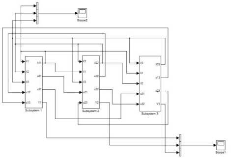
Fig. 6. Simulation Block Diagram of Linear Time-Delay System

C. SIMULINK Block Diagram and Simulation Results

As the whole system consists of three identical subsystems, therefore, block diagram of each subsystem is built first using Matlab SIMULINK. The block diagram of subsystem 1 is shown in Fig. 5 and the block diagram of the whole system is shown in Fig. 6.

The experimental procedures to determine different delay values were shown in [29], [30]. In this paper, the system is simulated by setting the initial condition as x 1 (0) = 0.85, x₂ (0) = 0.63, and x₃ (0) = 0.5;X 1 = 3ц 1 ,X 2 = 0, X 3 = 0; Ц 1 = ц 2 = Ц 3 = 1. Processing gain for all the subsystems is thought as equal, i.e., K₁ = K₂ = K₃ = K and all other conditions are same as in [5].

Fig.7 and 8 show the experimental responses as queue length vs. time with K₁ = K₂ = K₃ = 1000 and K₁ = K₂ = K 3 = 2000 respectively. On the other hand, Fig. 9 and 10 show the responses as (queue length-local average queue length) vs. time with K₁ = K₂ = K₃ = 1000 and K₁ = K 2 = K 3 = 2000 respectively.

It is observed from the simulation outcome that the oscillatory behaviour of system responses increased as the gain increased. At the same time we can see that, responses in Fig.8 and 10 with the higher gain oscillate more and die out slowly compared to responses in Fig.7 and 9 with less gain.

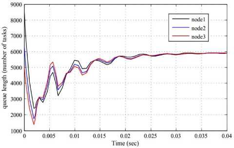
Fig. 7. Experimental responses as queue length vs. time with K1 = K2 = K3 = 1000

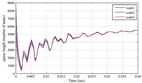
Fig. 8. Experimental responses as queue length vs. time with K1 = K2 = K3 = 2000

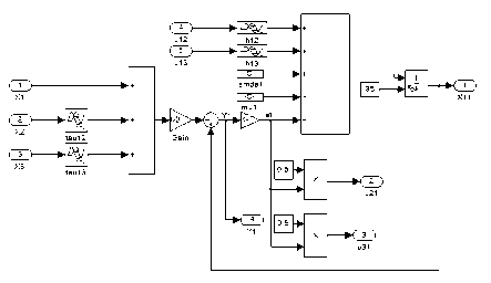
Fig. 5. Simulation Block Diagram of Subsystem 1

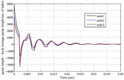
Fig. 9. Experimental responses as (queue length-local average queue length) vs. time with K1 = K2 = K3 = 1000

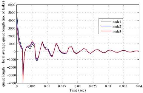
Fig. 10. Experimental responses as (queue length-local average queue length) vs. time with K1 = K2 = K3 = 2000

This unexpected behaviour is due to the delay experienced by the subsystems during communication. If delays are set to zero, then responses with higher gain will die out faster as expected. The oscillatory behaviour of the output responses depend on the linear control law (load balancing algorithm). The system experiences time delay whenever any transmission takes place among nodes. In the above system, transmission of task depends on the value of u i (t ) = - K i y i (t ) as decided by the linear control law. According to load balancing algorithm, if at the i-th node, - K i y i (t ) <  0, i.e., y i ( t ) >  Othen i - th node sends some of its tasks to other nodes. On the other hand, if y i ( t ) <  0, i.e., u i ( t ) = - K i y i (t ) >  0 then the node will not send tasks to other nodes rather the node is instantly takes waiting time (tasks) from other nodes.

• IV.    O bservers for L inear T ime - delay S ystems

In the previous section, a linear time-delay system is modelled and simulated to observe the effect of time delay on system performance as speed of load balancing operation and oscillatory behaviour of responses. In this section, observers of the linear time-delay system are designed considering the effect of time-delay in the system performance. The idea of an observer is that by merging calculated feedback signals with information of the modules of the control system, the behaviour of the system can be identified with higher accuracy as compared to utilising the feedback signal alone [16]. System performance can be improved by using an observer with skill and the reliability of the system can also be increased.

• A.    Mathematical Model of Observer

Let a time delay system be defined as follows:

X(t ) = A ( d ) X(t ) + Bu , y(t ) = C ( d ) X ( t )     (16)

where, X ( t ) e R ” is the system state and y ( t ) e m^m is the output of the system at time instant t . A ( d ) and

C ( d ) are polynomial matrices in the time-delay operators d = { d i } . For any i, operator ••; is defined by d i X(t ) = X(t - t) with т i >  0 which is the time-delay constant. When compared to the standard Luenberger observer, the following system might be considered as an observer for the system described by (16):

X ( t ) = A ( d ) X ( t ) + Bu + L ( d )( y (t ) - C ( d ) XX (t ))   (17)

where,  XX(t) ^ X(t)  as t ^^ for arbitrary initial values of Xˆ (t) and L(d) is the observer gain.

Now we can derive the definition of our system from (15) as follows:

X(t ) = X - ц + A ( d ) X(t ) and y(t ) = CX(t ))

Now by using observer design concept described in (17), the observer for the linear-time delay system considered in this paper can be defined as:

• XX ( t ) = A ( d ) J X ( t ) + X - ц + L ( d )( y - CX: (t ))     (18)

• B.    SIMULINK Block Diagram and Simulation Results for the System with Observer

  According to the observer equation and using SIMULINK built in blocks an observer is designed for subsystem 1. The block diagram for the observer of subsystem 1 is shown in Fig. 11. Fig. 12 and 13 show the responses of the system as queue length vs. time , and Fig. 14 and 15 show the responses as (queue length-local average queue length) vs. time in the presence of observer with system and observer gain K₁ = K₂ = K₃ = 1000, L = 1000, and K 1 = K 2 = K 3 = 2000, L = 2000 respectively.

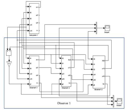
Fig. 11. Block Diagram of Observer 1 of Linear Time-Delay System

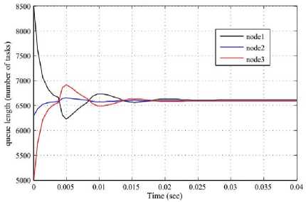
Fig. 12. System responses as queue length vs. time in the presence of observers with K1 = K2 = K3 = 1000 and L=1000

• V.    D iscussion

  

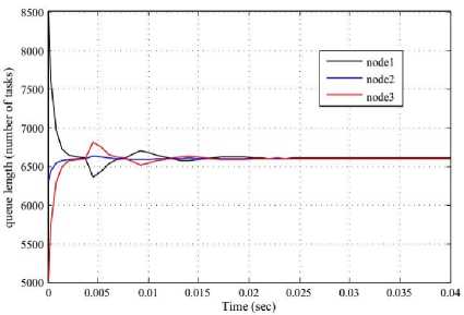
  Fig. 13. System responses as queue length vs. time in the presence of observers with K1 = K2 = K3 = 2000 and L=2000

  
  

One important issue in designing linear time-delay system is determining whether the system model is stable in the presence of oscillation in the system responses. It is well established that the presence of delays in various states of the system has an enormous impact on the stability of the system. Even if the system is stable, still system performance can be sluggish. For example, if the system is stable but oscillates too much while transferring tasks back and forth among subsystems rather than processing tasks, then system performance will degrade and the system will unnecessarily waste resources. Considering all possible issues with regard to stability and performance of the system, a linear time-delay system is modelled to observe the stability of the load balancing performance.

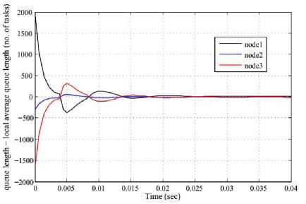
Fig. 14. System responses as (queue length-local average queue length) vs. time in the presence of observers with K1 = K2 = K3 = 1000 and L=1000

The system experiences delays during sending waiting time (queue size) and tasks from one subsystem to another. For simplicity, delays in sending queue size and tasks are considered as constant, but in real life usually delays are not constant. Initially, all the subsystems are fed with an equal quantity of load. Then subsystems experience creating and reducing waiting time. But, since the rate of reduction of the waiting time for all subsystems are we deliberately set as equal, i.e., Ц 1 = Ц 2 = Ц 3 = 1 and generation of waiting time as unequal, i.e., X 1 = 3p- 1 ,X 2 = OA 3 = 0 therefore loads become imbalanced within few moments. To balance loads among the nodes, each node shares load information with other nodes. As communications to share waiting time take place among nodes, all the nodes experience delays. As a result, subsystems receive queue size (expected waiting time) and tasks delayed by a certain amount of time.

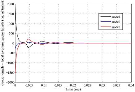
Fig. 15. System responses as (queue length-local average queue length) vs. time in the presence of observers with K1 = K2 = K3 = 2000 and L=2000

The linear control law и (t) = -Kiyi (t) is used for load balancing, where ui (t) is the reduction rate of waiting time xi (t) , and evaluated as per unit time. Here, the system gain K denotes the reduction rate of the waiting time of the system. According to the control law, within ∆t time period between consecutive executions of the load balancing algorithm, a fraction of the queue is removed resulting into reduced waiting time. According to the linear control law, with higher system gains, the waiting time reduces quickly. In the simulation, it is observed that with higher gain the system responses oscillate more and die out slowly. This unexpected system behaviour is due to the delays experienced during communication. If we can compensate the effect of delays on system performance, then the system responses will die out fast as expected with higher gain. As delays are unavoidable, therefore the system gain is chosen in a way that the system responses oscillate moderately and system performance are mildly affected. To avoid the effect of time delay during the exchange of waiting time, observers are designed for all subsystems. Observer of each subsystem can estimate some important information, and thus enabling each subsystem to work independently. As a result, communication between nodes to exchange waiting time is no more necessary; therefore no delay is experienced by the system due to communication.

• VI.    C onclusion

In this paper, a linear time-delay system is modelled to analyse stability and performance of the system in performing load balancing operation and observers of all subsystems are designed based on the analysis. It is assumed that the system consists of three symmetric subsystems and all the delays experienced by the subsystems are constant. In principle, system performance is considered as less oscillation in the responses and high throughput that increases as the system gain increases. Stability is another issue which requires to be considered along with system performance. In the modelled system, to perform load balancing operation each subsystem has to communicate with other subsystems to get information about the amount of load on other subsystems. This result in the system experiencing delays due to mutual communications between subsystems and these delays limit the value of the system gain.

It is observed that, the system responses oscillate more with higher gain in comparison to lower the gain. More oscillation in system responses means the system waste resources by passing tasks back and forth among subsystems rather processing tasks which results in degraded system performance. This unexpected behaviour of the system is due to the delays experienced by the subsystems while communicating with each other. After analysing system responses, observer of the system is designed keeping the effect of time-delay on system performance in mind. As observers are designed considering all the issues that affect system performance, therefore expected system performance, i.e., the load is balanced quickly with higher gain, is obtained from the system with the observer.

In this experiment, all the subsystems of the system were considered as symmetric and all the delays experienced by the system as constant. But in real life, it is not necessary for all the subsystems of a system to be symmetric and delays to be constant. Delays depend on different physical properties such as the availability and bandwidth of network, execution time of programs etc. Therefore, in future we plan to model linear time-delay system and design observers of the system considering variable delays and asymmetry of the subsystems. A processor of a subsystem uses a considerable amount of time to perform load balancing other than processing tasks which is not considered in this work. In future, the time required by the processors of the subsystems to perform load balancing operation can be taken into account together with the time required to process tasks.