Evaluation of reconstructed radio images techniques of CLEAN de-convolution methods

Deconvolution refers to the process of reconstructing a model of the sky brightness distribution given a dirty (Residual) image and the Point Spread Function (PSF) of the Instrument. [1] Under certain conditions, the Residual image can be written as the result of a convolution of the true sky brightness and the PSF as in the following formula. The CLEAN Algorithm is one of the most successful deconvolution procedures which are devised by Hogbom [3]. CLEAN applied numerically

Deconvolving process in the image (I, m) domain, CLEAN is an essential tool in producing images from incomplete (u,v) data sets , it converges to a solution that is the least mean square fit of the Fourier transforms of the delta-function components to the measured visibility [2] .

CLEAN based Hogbom is the first algorithm introduced for deconvolving Radio Images which represents the sky as a set of delta functions I_S k _y = £g_x 6(x) , Where g_x is the fixed loop gain and 6(x) is delta component .According to our evaluations, it is computationally efficient and it is very fast for small images. On the other hand, it is susceptible to errors due to inappropriate choices of imaging weights especially if the PSF has high side lobes. This is because of inappropriate preconditioning that will not be corrected during the major cycle and does not always produce satisfying results for extended sources in the following the detailed first CLEAN Algorithms introduced by Hogbom.

• - Convolution Equation

V (u,v) = JJI (i,m) e-2ni(ui,vm) .didm(1)

Vobs (U,V) = S (U,V)• V (U,V)

F [Vobs (U,V)] = F [S(U,V)• V (U,V)]

Iobs (i,m) = F-1 [S(u,v)]*F-1 [V(u,v)]

Iobs (i,m)= Ipsf (i,m) *Isky (i,m)

= JJ S (u, v) • V (u, v) e-2ni(ui-vm). dudv where I(i, m) is Sky brightness distribution, I(i, m)obs Observed sky distribution, I(i, m)sky is the true sky distribution, V(u, v) Interfometery response (visibility function), S (u,v) is Point Spread Function (sampling function) .The observed image is a convolution between the PSF and the true sky brightness distribution. Our deconvolution Problem is to separate the PSF from the sky brightness distribution with the dirty image and to estimate spatial frequencies in unmeasured regions of the UV plane.Detailed Comparative Study is required to evaluate CLEAN Variants based Reconstruction Radio Images for further Performance Enhancement, especially with Compressive Sensing New Techniques that is growing rapidly for updated challenges as Big Data Radio interferometric Imaging [22].

• II.    Materials and Methods

I used real measurement Set for Evaluation of CLEAN Variants. The supernova remnant G055.7+3.4 data set will be evaluated under Single field deconvolution (Hogbom, Clark, Clark Stokes and Cotton Schwab) and wide filed deconvolution (Multi Scale, Multi Frequency and Multi Scale Multi frequency).

• A.    CLEAN Hogbom Algorithm

At the beginning, we must describe in details the First Algorithm of the CLEAN Variants (Hogbom) as the following algorithms that are derived from HOGBOM [3] CLEAN. Whereas the input is the dirty image, PSF; the parameters are: gain, iterations limit, Flux Threshold, and the Output: Sky model, Residual image, Restored image. The algorithm can be described as follows:

• 1.    Make a copy of the dirty image i_d ( i , _m ) called the residual image I_R ( i , m ) .

• 2.    Find the maximum pixel value and position of the maximum in the Residual image I_R ( i , m ) .

• 3.    Subtract the PSF Multiplied by the Peak pixel value f_max and gain factor g from the Residual image I_R ( i , m ) at the position of the peak I R + 1 = I R - g " B " m ^ax( I »)'

• 4.    Record the position and the magnitude of the point source subtracted in a model gf .

• 5.    Go to (step 2). Unless all remaining pixel values are below some user specified threshold or the number of iterations have reached some user specified limit.

• 6.    Convolve the accumulated point source sky model with a restoring beam, termed the CLEAN beam (usually a 2-D Gaussian fit to the main lobe of the PSF.

• 7.    Add the remainder of the Residual image I_R ( i , _m ) to the CLEAN image formed in (step 6) to form the final restored image.

max

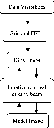
Fig.1. Hogbom CLEAN

• B.    CLARK CLEAN Algorithm

The rise of CLEAN has been the continuing efforts to improve computational speed of CLARK CLEAN [4] . Clark CLEAN took optimal advantage of FFT and the use of Speed Processors [4]. Clark Algorithm has the advantage of involving much more computations. It has less effort to implement compared to Hogbom and this not only means reduction of the computational load but also elimination of aliasing errors [5]. It uses PSF patches for updates and calculates residuals by using gridded visibilities. This procedure is divided into major and minor cycles that will be shown in the Fig.(2).

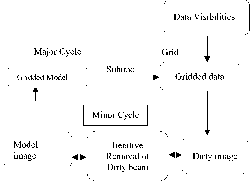
Fig.2. Clark CLEAN

• C.    Cotton Schwab CLEAN Algorithm

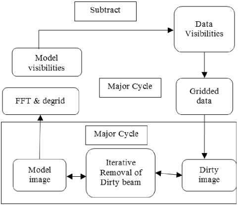
The cotton-Schwab [6] presents an alternative to the standard CLEAN Algorithm, predicts highly periodically model-visibilities without pixilation errors, calculates residual visibilities and re-grids major and minor cycles without errors as shown in fig.(3).

CLEAN Algorithms consists of two different categories first one operates with a delta function sky model as the pervious algorithms and others with a multi-scale sky model.

• D.    Multi-Scale CLEAN Algorithm

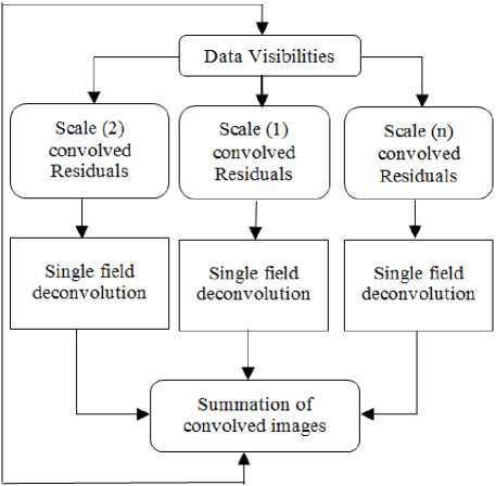
Multi-Scale CLEAN (CH-MSCLEAN) [7] is a scalesensitive deconvolution algorithm which is designed for images with complicated spatial structure. It parameterizes the image into a collection of inverted tapered paraboloids. The minor cycle iterations use a matched-filtering technique to measure the location, amplitude and scale of the dominant flux component in each iteration, and take into account the nonorthogonality of the scale basis functions while performing updates. It represents the sky as a set of Gaussians.

shpmod

I sky = 2 Is * Is where I^ is a blob of size of different scale sizes, imodciis a set of delta function imodel =I gs^ (i _ is,i )

From eq. (6) it clearly appears that Multi-scale Algorithm is just Summation of Multiple Scale of the Single Field deconvolution Output Algorithm [6] as it shown in the following figure.

The Advantage of using Multi-scale: (i) Improving convergence and stability. (ii) Finding and detecting emission on the largest scales first, moving to finer and finer detail as iteration proceeds. (iii) Converges to relatively stable values of the flux on different scale.(iv)Much better reconstruction of extended sources than single-scale CLEAN.(v) Efficient representation of both compact and extended structure (sparse basis).(vi) Naturally detecting and removing the scale with maximum power.(vii) The implementation efficiency of CLEAN is retained (model and residual updates). (viii) This method could use any basis set to bias the reconstruction (shape lets). (ix) Can use higher loopgains than with CLEAN because the model is more accurate. In general, we can see the benefits of using Multi-Scale Method, however there is a different technique of using measurements at several observing frequencies when forming an image in radio intereferometric aperture synthesis.

v - v

v

sky          sky

I v = / I t t

whereI_£ ^sky a set of delta function is, I^is sky brightness, v is observing frequencies .This Technique is called Multi-Frequency synthesis (MFS) which means gridding different frequencies on the same UV grid [8] Using this method gives great aperture filling and thus cleaner dirty beams. The more data we can process using MFS, the better Signal to Noise Ratio (SNR) The drawback of this method is that it uses huge database for wide band observations .This leads to 'holes' around sources due to average PSF Subtraction and MFS breakdown of assumption of mono-chromaticity.

There is a new approach to multi-frequency synthesis in radio astronomy by using Bayesian Inference Technique [9]. This technique estimates the sky brightness and the spectral index simultaneously by merging both multi-frequency high resolution imaging and spectral analysis. This approach is called (Resolve) [9] and works under the assumption that the extended surface brightness at a single frequency is a priori assumed as a random field drawn from log normal statistics. For our multi-frequency problem dv = IR + П            (9)

It turns (9) into dv = Rv [I°(i, m, v°)] + nv s i,m

= Rv [ p°e )] + nv

where s is where s is a Gaussian random, and p « is a constant to normalize the system to the right units. There always new attempts to get better performance like MUFFIN [10] which focuses on the challenging task of automatically finding the optimal regularization parameter values. However, this new approaches for the MFS Method make combination of two well performed methods Multi-scale and Multi-frequency.

Multi- scale Multi-Frequency CLEAN Deconvolution [11] represents sky brightness distribution as a collection of multi-scale flux components whose amplitudes follow a Taylor-polynomial in frequency). The MS-MFS algorithm models the wide-band sky-brightness distribution as a linear combination of spatial and spectral basis functions, and performs imagereconstruction by combining a linear-least-squares approach with iterative χ2 minimization. This method extends and combines the ideas used in the MS-CLEAN and MF-CLEAN algorithms for multi-scale and multifrequency deconvolution respectively, and can be used in conjunction with existing wide-field imaging algorithms.

Ivk =VIt (v-vi t)(11)

.

i.=S[ i* * i., ]

s where Isky represents a collection of δ-functions, represents I a multi-scale Taylor coefficient image, Ishp spatial-frequency-domain multiplication, the MS-MF Method has many benefits over previous ones:

(i)Minimizing imaging artifacts achieve continuum sensitivity and reconstruct spatial and spectral structure at the angular-resolution which is allowed by the highest observed frequency.

• (ii)    This algorithm achieves dynamic ranges >10^5 on test observations with the EVLA, and dynamic ranges >10^6 on noise-free simulations.

• (iii)    For sources with smooth continuum spectra, it is able to reconstruct spectral information at the angular resolution allowed by the combined multi-frequency u-v coverage.

The drawbacks of using MS-MF Method:

(i)MS-MFS are inefficient in memory use, and other approaches may be required for large image sizes.

(ii)For full-Stokes wide-band imaging, where a Taylor-polynomial in frequency is not the most appropriate basis function to model Stokes Q, U, V emission, wide-band imaging with other flux models must be tried. After describing Deconvolution based CLEAN Algorithms, we will make some tests over these methods.

• III.    Performance Metrics

The CLEAN Algorithms have been tested using I test CLEAN Algorithms over Time, Root Mean Square Error (RMS), Standard deviation (STD), flux density and Dynamic Range (DR) [12, 23]. The dynamic range of an image is usually defined as the ratio of the maximum Intensity to the RMS level at some part of the field where the background is mainly Blank sky. Achieving high dynamic range requires advanced calibration and proper imaging.

Dynamic Range = Flux Density / RMS (noise) (13)

where RMS is a measure of how concentrated the data is around the line of best fit, computed as described [13] in the following equation.

RMS = .l^¹^^{2              (14)}

n where 12 squares of the pixel values, n is the pixels number, also we can compute the Standard deviation of the mean (STD) [14] as in the following equation.

()2

(n-1)

We also compute the time which the algorithm takes to perform cleaning Process.

• IV.    Results and Discussion

• A. Experiment Setup

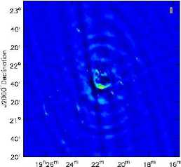
  We use calibrated data which are taken with the Karl G. Jansky Very Large Array, of a supernova remnant G055.7+3.4. [21] The data were taken on August 23, 2010, in the following figure (1) shown the G55 with No deconvolution just Fast Fourier Transform (FFT).

J2000 Right Ascension

Fig.5. G55

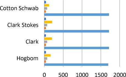
Using Common Astronomy Software Applications (CASA) Program to evaluate the CLEAN Variants for both Single field Algorithms in table (1) and Wide field deconvolution in table (2) Under Xeon, 64 bit 2.8 GHz Processor and Red Hat Enterprise Linux operating system .

B. Simulation Results

Table 1. Single Field Deconvolution

0» я	7	1 я	и	о и	1 я и
5 £	DR (Jy)	577.4630	462.2018	462.2018   4	62.2018
	RMS (µJy)	159.33	150.94	150.94	150.94
	Flux density (kJy)	92.00718	69.76475	69.76475	69.76475
	Time (S)	189	197	193	154
	STD (µJy)	159.32	150.93	150.93	150.93
Я .О я D	DR (Jy)	1710.459	1763.756	1705.420	1705.420
	RMS (µJy)	39.12823	39.17514	39.12788	42.90252
	Flux density (kJy)	66.92727	69.09541	66.72952	66.72952
	Time (S)	209	185	206	245
	STD (µJy)	39.12528	39.17200	39.12495	39.12495
«	DR (Jy)	1697.838	1717.092	1717.092	1717.092
	RMS (µJy)	44.16861	44.15866	44.15866	44.15866
	Flux density (kJy)	76.00987	75.82453	75.82453	75.82453
	Time (S)	166	204	207	128
	STD (µJy)	44.16311	44.15319	44.153196	44.15319

Table 2.Wide Field Deconvolution

0» я	2	S	.Д Я	। а S
5	DR (Jy)	666.1691	464.9499	322.3489
	RMS (µJy)	122.46	209.62	119.75
	Flux density (kJy)	81.57908	95.3666	38.60129
	Time (S)	1056	183	962
	STD (µJy)	122.45	209.62	119.75
,о я D	DR (Jy)	4194.61415	1323.67790 8	3956.716782
	RMS (µJy)	42.90252	51.00450	52.491892
	Flux density (kJy)	179.9595	67.51353	207.69555
	Time (S)	182	159	1152
	STD (µJy)	42.88296	51.00231	52.476605
	DR (Jy)	3548.078	1253.084	3401.3176
	RMS (µJy)	48.1849	62.39434	58.470466
	Flux density (kJy)	170.9638	78.1854	198.87663
	Time (S)	194	121	1177
	STD (µJy)	48.15938	62.39023	58.442003

■ STD ■ Time ■ Flux Density ■ RMS ■ DR

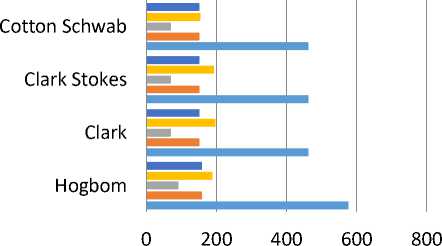
Fig.6. Natural Weighting Single Field

Multi Scale Multi Frequency

Multi Frequency

Multi Scale

■ STD ■ Time ■ Flux Density ■ RMS ■ DR

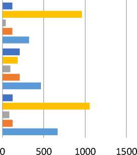
Fig.7.Natural Weighting Wide Field

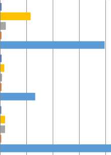
The Natural gives constant weights to all Visibilities and gives optimum point source sensitivity in an image from Fig. (6) for single field algorithms, the calculations for Hogbom Algorithm has better performance when it comes to DR. On the other hand, residual algorithms have the lower DR which indicates that the simple structure of Hogbom when operating with delta functions is optimal, but it depends also on the right choice of the image weighting; however Hogbom has one of the highest processing time, accordingly The best processing time is in cotton Schwab due to its ability to clean many separate but proximate fields simultaneously .the highest error deviation is in Hogbom which indicated that some data are far from the regression line data points. Hogbom has the better performance in flux density than the other methods. From Fig. (7) For wide field algorithms, Multi scale has the best performance in DR due to better reconstruction than classics methods and Converges to relatively stable values of the flux on different scale .Multi Scale multi frequency has the lowest DR because of its complex structure and needs to be run over bigger images, On the other hand, MSMF has the lowest error deviation as a result of Minimizing imaging artifacts achieve continuum sensitivity. The flux density for multi frequency is much bigger than MS and MSMF which effects on the quality of the radio image, on the other hand the lower Flux density belongs to MSMF that use to work with complex and Extended Images to gain better flux density . the MF has the smallest Time for wide field imaging that’s because its ability to observe several frequencies simultaneously and avoiding bandwidth smearing by uses the correct frequency of every sample of the visibility function rather than some average frequency.

Cotton Schwab

Clark Stokes

Clark

Hogbom

• ■    STD ■ Time ■ Flux Density ■ RMS ■ DR

  Multi Scale Multi Frequency

  Multi Frequency

  Multi Scale

  
  
  

  0  1000 2000 3000 4000 5000

• ■    STD ■ Time ■ Flux Density ■ RMS ■ DR

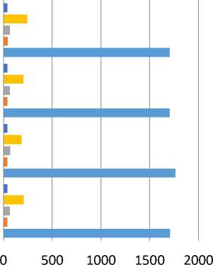
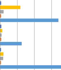
Fig.9. Uniform Weighting Wide Field

In general The Uniform Weighting gives weight inversely proportional to the sampling density function which affects the behavior of the operating algorithm making best resolution but higher noise and gives better angular resolution at the expense of sensitivity since low spatial frequencies are weighted down and the data are not utilized optimally. In particular we can see that Clark has the highest dynamic range, highest flux density and lower time consumption of the running algorithm by set iterations of hogbom minor cycle using small patch of the PSF .Hogbom has the lowest DR because it susceptible to errors due to inappropriate choice of imaging weights, especially if the PSF has high side lobes, however the four methods for single field deconvolution have almost the same result as shown in Fig. (8) Which indicates that uniform weighting has stable behavior as we follow in uniform the eq.(16) .

1 w=

where W is weight of the visibility . This formula makes even visibilities all over the grid. Cotton Schwab has the highest time under uniform weighting. For wide field imaging Fig. (9) Shows that Multi Scale has the best DR and lowest error deviation because Multi scale built for Improving convergence and stability and to deal with extended sources, while Multi scale Multi frequency has the highest flux density for uniform weighting by Minimizing imaging artifacts achieve continuum sensitivity, Multi frequency has the smallest processing time but normal performance when it comes to DR, Flux Density and error deviation.

Fig.8.Uniform Weighting Single Field

STD Time Flux density RMS DR

Fig.10. Briggs Weighting Single Field

Multi Frequency

Multi Scale

Multi Scale Multi Frequency

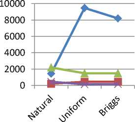
Clark Stokes and Cotton Schwab have the highest results. Cotton Schwab has the smallest time of processing and Clark Stokes has the biggest time. From Fig. (11) For wide field deconvolution, Multi scale has the best DR and lowest error deviation, while MSMF has the highest flux density and biggest Processing time.

• V.    Discussions

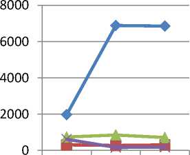
The different measurements that we took for single field deconvolution from table (1) clarify that Results changes by Weighting Types (Natural, Uniform and Briggs), from observing the results there are slightly difference when it comes to the DR and RMS. On the other hand, it changes slightly large when it comes to Time which Clearly which appears in Cotton Schwab. The Differences that form the Weighting appear clearly and show that Briggs Weightings [15] is the Best performance among the other two types for the Single Field Methods. We can say that wide field deconvolution results from table (2) has much bigger DR when it comes to the Three Methods MS, MF and MSMF, especially for Uniform and Briggs Weighting, as for time both MS and MSFS have lower time for the Natural Weighting, MF has less time for uniform Weighting, The lower RMS for MS, MF and MFS is in uniform Weighting, finally all these differences appears in the following figures

STD Time

0   1000 2000 3000 4000

Flux Density RMS DR

Briggs Weighting is optimal combination of two weighting scheme Uniform and Natural Weighting with a sliding scale based on the signal to noise ratio of the measurement and a tunable parameter that defines a noise threshold to derive new weighting scheme has an adjustable parameter that allows for continuous variation between the maximum point source sensitivity and the highest angular resolution ,Briggs creates a PSF that smoothly when weight density is high the effective weight to use is uniform and following the eq.(17)

u , v

, u,v                     2

1    + w f u,w

2   (5*10-R )2

2 w u,v       u,v w u,v u,v

Natural Uniform Briggs

DR

Flux Density

Time

Error deviation

Fig.12. Weighting Comparison for Single field

DR

Flux Density

Time

Error deviation

where w is weight of visibility , R is a robust parameter

From Fig. (10) For single field, we figure that Hogbom has the lowest DR for Briggs weighting, while

Fig.13.Weighting comparison for wide field

Using Multiple weights for reconstruction process on supernova remnant G055.7+3.4. From fig. (12) Appears that uniform weight has the best performance over other weighting methods, best flux density from Briggs Weight, less time for Briggs Weight and less error from uniform weight.

Weighting schemes produces different measurement for MS, MF and MSMF. The best DR for the share of uniform weighting, in addition of best flux density and less error deviation, Briggs weight has the less time consumption.

• VI.    Conclusions and Suggested Future Work