Evolutionary algorithm with an autoencoder-based dimensionality reduction mechanism

In contemporary applied optimization, problems are frequently set up as black-box models, where objective functions are evaluated algorithmically or via simulation modeling. These problems typically lack information on the function's behavior or are too complex for conventional analytical methods. The growing complexity of such problems has driven the creation of new techniques, such as direct search algorithms and metaheuristics. Among the most prominent and effective approaches for blackbox global optimization are evolutionary algorithms (EAs), which are stochastic population-based methods inspired by evolutionary biology processes [1]. Due to their active development and promising performance, EAs are widely used for solving applied problems [2]. Nonetheless, applying EAs to specific problem types is still difficult because of their high computational expense and sensitivity to dimensionality.

A common strategy to mitigate the mentioned limitations is to combine optimization methods with approximation techniques. Surrogate modelling is a widely adopted approach for computationally expensive problems. In surrogate-assisted Evolutionary Algorithms (EAs), these models serve as lowcost approximations of the fitness landscape. They allow the estimation of candidate solution quality, reducing the number of costly fitness function evaluations (FEs). Commonly used surrogate models include Random Forests [3], Gaussian processes [4], and Radial Basis Function networks [5]. However, as the problem dimensionality increases, building an adequate model requires an impractically large amount of data, leading to a decline in the optimization algorithm's efficiency.

Several strategies have been proposed to overcome the «curse of dimensionality». One of the research directions employs decomposition-based approaches, which break down the problem into simpler and independently optimized subproblems [6]. Another direction focuses on introducing specialized genetic operators combined with local search [7]. While such methods can often mitigate the impact of high dimensionality, they often rely on the separability of the problem or its specific properties, their effectiveness depends on problem-specific properties like separability, which can complicate the construction of surrogate models. As an alternative, unsupervised learning methods, particularly dimensionality reduction techniques, can be employed to reconstruct the search space. In addition to classical techniques like Principal Component Analysis (PCA), autoencoder-based methods can be adopted.

This work proposes an evolutionary optimization framework with autoencoder-based dynamic learning. In this approach, autoencoders are utilized to identify dependencies in the fitness landscape by constructing corresponding latent spaces from populations obtained during optimization. The concurrent operation of optimizers in the original and compressed spaces facilitates a more efficient search. The performance of the proposed algorithm is evaluated on a set of benchmark problems, an analysis of convergence and population dynamics at various stages is presented.

Problem statement

A continuous global minimization problem can be stated as follows:

f(x)→min,f :Rn→R, x∈Rn where f(x) is an objective function, vector X = (x1, …, xn), xi ∈ S defines an arbitrary solution in n-dimensional space. The search space S is defined by a hypercube with lower bounds lbi and upper bounds ubi. The solution to problem (1), or global minimum, is a vector x*∈ S such that∀x∈S: f (x*) ≤ f (x). The computational budget for evaluating the objective function is moderate, meaning it is too small to employ standard evolutionary algorithms (EAs) but sufficient to explore methods beyond simple local descent.

This work considers a black-box setting, where the properties and derivatives of f ( x ) are unknown or difficult to interpret; only a set of input vectors and the corresponding output values can be considered by optimizer during the search process. This characteristic typically makes the use of mathematical optimization methods difficult, making heuristic and metaheuristic algorithms a practical alternative. While their performance is not strictly guaranteed, it is often sufficient for practical applications. One of the most popular approaches for solving black-box global optimization problems are evolutionary algorithms.

Evolutionary Algorithms (EAs) are population-based optimization approaches inspired by biological evolution. Each new generation is created by applying genetic operators to existing individuals, iteratively updating the population through the selection of superior solutions and random variations. A fitness function is used to evaluate solutions, which is typically identical to the objective function but may also incorporate additional problem-specific requirements. Throughout the development of the field, a large number of evolutionary methods have been proposed, many of which specialize in problems with specific variable types or problem formulations. The family of Differential Evolution (DE) algorithms is considered one of the most effective approaches for continuous optimization.

Success History-based Differential Evolution

The Differential Evolution algorithm was introduced by Storn and Price in 1995 [7]. The classical version of DE begins by initializing a random population of size N. For each individual, the value of the objective function is evaluated. The algorithm then proceeds through an iterative cycle of genera- tions. Its key mechanism is the mutation operator, which generates new candidate solutions. A classic strategy, denoted as rand/1, is defined by the following expression:

^V ij    x r- 1 j + ^{F (} x r 2 j    x r 3 j ) ^,

where V ij is a mutant vector, r 1, r 2, r 3 are randomly chosen indices ( r 1 ≠ r 2 ≠ r 3), i is the index of the current individual, j is the variable index, F is a scaling parameter. If the j -th coordinate value violates the search space boundaries, a random value is generated as a replacement. The crossover operator is then applied to the resulting mutant vector. The most commonly used scheme is binomial crossover ( bin ), defined as follows:

u ij

'Vy, if r <  CRorj = jr , x jj , otherwise ,

where u i is a trial vector, CR is the crossover probability, CR ∈ [0;1], jr is a randomly selected index from [1; n ], ensuring that at least one coordinate of the mutant vector is changed.

Next, the trial vector is compared to the parent individual with the same index i . In case of minimization, if the trial vector has a lower objective function value, it replaces the parent individual. This procedure is known as selection and is defined as:

u ij

u j , ^{f f} ( u j ) < ^f ( x j ) , x .. , otherwise.

These three operators are applied in sequence to generate each new population. Then the next cycle starts with new individuals. The algorithm repeats this sequence until user-defined termination criteria are met, usually the limit of FEs or working time. A notable limitation of this approach is the need to manually tune parameters ( N , F , CR ), as well as to select a mutation strategy. To address these issues, numerous heuristics have been proposed to enhance search efficiency, including self-adaptive parameter control mechanisms [9, 10].

The L-SRTDE algorithm is a DE modification proposed by Stanovov and Semenkin for the 2024 IEEE CEC special session [11]. This method employs two populations of equal size, one maintaining the best-found solutions ( x^top ) and the other containing new solutions ( x^new ). During the initialization phase, both populations are filled with identical solutions. It employs a mutation strategy denoted as r-new-to-ptop/n/t , which is formalized as follows:

new        top        new         new top

V ij = x r 1, j + F ( x pbest , j    ^x i, j ) + F ( x r 2, j    x r 3, j ) ,

where r1, r2, r3 are randomly selected indices ( r1 ≠ r3 ), index r2 is selected via rank-based selection with selective pressure; pbest is a randomly selected index from the top pb % best solutions. The selection step is formalized as follows:

xnc

= u j ,iff ( u j ) < f ( x nw ) , x_nc, otherwise,

where nc is an index that increments after each successful selection. The population is then updated by ranking individuals based on fitness function values and applying a linear population size reduction. The scale factor F is controlled using the Success Rate measure: SR = NS/NP , where NS counts the number of successful selection runs during the current generation. The expected value of the parameter is calculated as mF = 0.4 + 0.25 ∙ tanh (5 ∙ SR) . The elite proportion pb is determined by

pb = max ( 2,0.7 e 7 ' SR ) . For the

crossover probability, a memory archive is used which contains re- cently successful parameter values.

Dimensionality reduction based on autoencoders

An autoencoder is an unsupervised feedforward neural network designed to learn efficient representations of input data by learning to reconstruct it at the output layer. A generalized structure of an autoencoder is presented in Fig. 1.

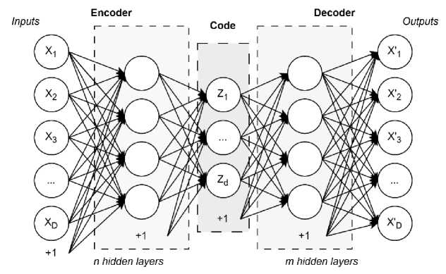
Рис. 1. Обобщённая структура автоэнкодера

Fig. 1. General structure of an autoencoder

An autoencoder consists of three components: an encoder, a code (or bottleneck), and a decoder. While the input and output layers have matching dimensionality, the central code layer usually has a purposefully reduced dimension. The encoder function g transforms the input into a code c ( x ), the decoder f then attempts to reconstruct the original signal from this code. The network is trained by minimizing the loss function L , which typically is a measure of reconstruction error between the input x and reconstruction f ( g ( x )).

Consider an autoencoder where Z j is the j -th neuron in its bottleneck layer, j = 1, d. The d -dimensional latent search space Z with encoding and decoding operations is defined. For an architecture with k₁ encoder and k₂ decoder hidden layers, the activation of a bottleneck neuron is given by:

Z j = f a n + £ ( x i , w n ) ,

\ i

where f is the activation function, aⁿ_j and w_iⁿ are the bias and weight parameters of the of n -th layer of the encoder, x_iⁿ are the outputs from the previous layer.

The reconstruction of the input is computed using the following equation:

'

x , = f a \

' m +

i

^

( z i , w i ) ,

where a ^' _j ^m and w_i ^{' m} are the bias and weight parameters of m -th layer of the decoder, x_i^m are outputs of the previous layer.

Autoencoders' capacity for dimensionality reduction is well-established in applications like frequency analysis, data filtering, and pre-training [12; 13]. Key advantages over alternative methods are their ability to extract non-linear sub-spaces and their potential for computationally efficient finetuning. These capabilities could be beneficial in evolutionary optimization, where they could be used to compress the search space into a more manageable and informative representation. Nevertheless, the integration of autoencoders with EAs currently remains an under-explored research area.

Among the key studies: Cui et al. [14] proposed a cooperative coevolutionary algorithm to orchestrate the interaction between EAs operating in the original and latent spaces; Hu et al. [15] explored their compression capabilities for dimensionality reduction in multi-objective large-scale global optimization problems. Both studies have shown promising results in effective search space compression based on population data. This work exploits this particular feature to dynamically reconfigure the compressed latent space throughout the optimization process, thus adapting the algorithm to each evolution stage.

Proposed framework

The complete algorithm is outlined in Fig. 2. During initialization, hyperparameters are selected, and a large initial sample of size N_init is generated using Latin Hypercube Sampling (LHS) [16]. The top N individuals from this sample are selected to form an initial population and used to train the autoencoder. Since autoencoders learn from unlabeled data, using a fitness-biased sample is more effective than a random one, as it provides a problem-relevant dimensionality reduction, which may lead to faster convergence in early generations.

The iteration process generally contains of three stages: 1) dynamic autoencoder training, 2) optimization in the latent search space and 3) optimization in the main search space. First, the autoencoder is retrained on the population P gained from the previous iteration. The updated model defines a latent search space with new bounds and a decoding mechanism. An evolutionary algorithm is used to evolve a randomly generated population in reduces search space, with the resulting population P_AE . Next, P is optimized in the original, high-dimensional search space, yielding the population P O . Finally, the combined offspring population P is formed, the number of FEs is redistributed between the component algorithms. If the stopping criterion isn’t met, the described steps are repeated with the new individuals.

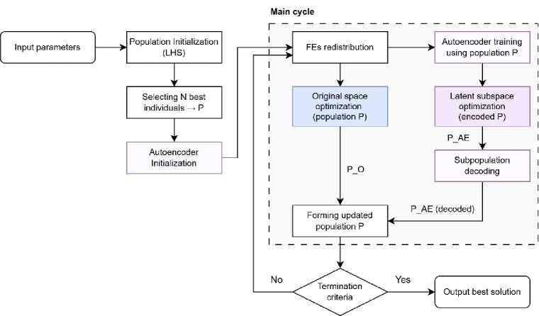
Рис. 2. Блок-схема предложенного алгоритма

Fig. 2. A flowchart of the proposed algorithm

Within the evolutionary process, the role of autoencoder is to compress the search space into a representation that facilitates more efficient exploration. By mapping topological structures of the original fitness landscape into a latent space, a well-configured autoencoder can accelerate the search for promising areas. Prior research on EA-assisted autoencoders [14; 15] typically involved a single training phase due to computational constraints, which makes the model's performance critically dependent on its initial state. To overcome these limitations, this work employs an iterative retraining strategy of the autoencoder during the optimization process.

The autoencoder training process starts by initializing a neural network with a specified structure. The input is the current population, and the data are normalized if required. Training is performed using the Adam optimizer over a set number of iterations. The boundaries of the latent space are adjusted based on the input data. From the trained network, a new latent-space objective function f_LT ( z ) is constructed, incorporating encoding and decoding operations. The code dimensionality is set by parameter d , and its impact on the algorithm's performance is explored in the next section.

The loss function is defined as the mean square error between input x and its reconstruction x' :

n ₂

Loss ( x ) = -M Xi ^- x ' ) ,                                ⁽⁹⁾

nl ~ 1

The description of the proposed algorithm (denoted as AEDE) in pseudocode is presented in Table 1. The parameters FEs AE and FEs O stand for latent and original problem function evaluations respectively and represent a number of FEs for each of optimization algorithm instances, FEs AE + FEs O = cFEs . These two metrics allow for controlling the balance of the search effort between the latent and original spaces. Also, the following adaptive scheme for computational resource allocation was proposed:

FEs AE

. I cFEs 1 0.25 FEs

= min I------,---

I 10 4 maxFEs

FEs O = cFEs - FEs_AE ,

where FEs is the current number of function evaluations, maxFEs is a maximum number of FEs, used as a termination criterion.

Table 1

The proposed algorithm (AEDE)

Inputs: D : problem dimension, lb , ub: problem bounds , N_init : initial sample size; a : autoencoder configuration, cFEs : the number of FEs per cycle, maxFEs : the maximum number of function evaluations.

Outputs: x^* : best solution, f ( x^* ): best fitness

1	Generate an initial sample S of size Ninit using LHS;
2	Calctulate f ( S );
3	Sort S by f ( S ) values , select N best individuals, form population P ;
4	while ( FEs < max FEs ) do
5	Train an autoencoder using P ;
6	Calculate FEs AE and FEs O by equation (10);
7	Run the optimization algorithm in latent subspace;
8	Run the optimization algorithm in original search space;
9	Sort PAE and PO ;
10	Form new population P by equation (11);
11	Update the best individual and its fitness value: x* , f ( x* );
12	end

The search is conducted independently within the original and latent spaces. The optimizer operating in the original space retains accumulated knowledge, utilizing the population from the prior iteration and maintaining its adaptive parameters. In contrast, optimization within the latent space involves resetting the algorithm's configuration. This design is motivated by the fact that the objective function landscape in the latent space changes after the model is retrained.

The populations resulting from the evolutionary search are combined using the following rule:

P = (PO ^PaeL/n-)Ln+na , where the notation |k / l defines the selection of the top k / l fraction of a population ranked by fitness, na is selected as

10 N . This selective integration is necessary to constrain the influence of the latent space, which, being a compressed representation of the original domain, spans only a limited region. Limiting its representation in combined population prevents premature convergence and maintains diversity.

The cycle then either proceeds to the next iteration or terminates if the stopping criterion is met.

Numerical experiments and analysis

This section presents the description and results of the experiments. The effectiveness of the proposed approach was evaluated on CEC 2017 and CEC 2022 benchmark global optimization problems [17; 18]. The study is divided into two stages: an investigation of the impact of latent space dimensionality on the algorithm's efficiency, and a comparison of the proposed algorithm with L-SRTDE under a moderate computational budget. The problems dimensionalities are 20 and 100, the performance was evaluated on a series of 30 independent runs.

To preserve the properties of the subpopulation optimization algorithm, the framework is extended with a linear population reduction mechanism, similar to that in L-SRTDE. The population size is reduced based on the current total function evaluation count. While the main space optimizer applies this rule on every cycle without an internal counter, the latent space optimizer restarts its reduction process following each autoencoder retraining. This proposed algorithm is denoted as L-AEDE.

The initial population size is set to 200 for all problems and dimensionalities. The minimum popu- lation size is set to 4 for the main space optimizer and

1 _N

for the compressed space optimizer.

The number of training epochs for the autoencoder is 200 for the initial training and 100 within the cycle. The size of the initial sample generated via LHS is 500. Unspecified L-SRTDE parameters were set as recommended by its authors. The encoder structure is {64,32}, the decoder structure is {32,64}, the activation function for hidden layers is ELU. The algorithm's performance was evaluated using standard deviation, the best value, mean value, and median value from the series of independent runs. The statistical significance of differences in experimental results was assessed using Wilcoxon’s signed rank test with a significance level α = 0.05.

The performance of L-AEDE on three distinct problems from CEC 2017 benchmark suite is summarized in Tables 2–3, with a computational budget of 100000 function evaluations for different latent space dimensionalities d. The first column denotes the benchmark problems and dimensionality of the original problem, while the subsequent columns demonstrate the algorithm's performance metrics.

As shown in Tables 2–3, none of the considered code sizes prevails among the tested configurations, confirming the parameter's problem-specific nature. However, the choice of code dimensionality still may affect problem-solving efficiency at different algorithmic stages. The convergence plots for different d values are presented in Fig. 3, where the horizontal axis indicates function evaluations and the vertical axis indicates the current best solution per subpopulation. It can be seen that the objective value disparities between the original and latent space populations during early optimization phases.

These differences become less noticeable as the algorithm progresses, which can be attributed to increased local convergence behavior. Fig. 4 displays convergence plots after applying the cumulative minimum operation, demonstrating the evolution of the best-found solution relative to both populations.

Optimization results of L-AEDE with different latent space dimensionality (min and median)

Table 2

Problem, D	d = 5		d = 10		d = 20
	Min	Median	Min	Median	Min	Median
f 1 , 20	1.000e+02	6.201e+02	1.019e+02	1.061e+03	–	–
f 6 , 20	6.000e+02	6.000e+02	6.000e+02	6.000e+02	–	–
f 25 , 20	2.910e+03	2.913e+03	2.910e+03	2.913e+03	–	–
f 1 , 100	3.355e+09	8.420e+09	4.798e+09	1.108e+10	2.519e+09	1.141e+10
f 6 , 100	6.164e+02	6.235e+02	6.166e+02	6.232e+02	6.171e+02	6.240e+02
f 25 , 100	3.547e+03	3.676e+03	3.538e+03	3.655e+03	3.559e+03	3.671e+03

Table 3

Optimization results of L-AEDE with different latent space dimensionality (mean and standard deviation)

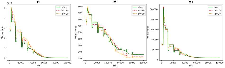
Рис. 3. Графики сходимости алгоритма для разного размера кода для задач размерности 100 (относительно субпопуляций)

Problem, D	d = 5		d = 10		d = 20
	Mean	Std	Mean	Std	Mean	Std
f 1 , 20	2.493e+03	3.113e+03	2.071e+03	2.746e+03	–	–
f 6 , 20	6.000e+02	3.872e-02	6.000e+02	3.893e-02	–	–
f 25 , 20	2.913e+03	7.465e-01	2.912e+03	1.027e+00	–	–
f 1 , 100	9.397e+09	5.040e+09	1.379e+10	7.038e+09	1.178e+10	5.522e+09
f 6 , 100	6.233e+02	3.434e+00	6.226e+02	3.388e+00	6.239e+02	3.319e+00
f 25 , 100	3.687e+03	9.210e+01	3.666e+03	8.618e+01	3.680e+03	7.721e+01

Fig. 3. Convergence graphs comparison for different code dimensionality on 100D medium-budget problems relative to subpopulations

Next, a comparative analysis is conducted between the proposed L-AEDE approach and the underlying optimization algorithm used in the framework (L-SRTDE). To investigate the impact of population reduction on method performance, two algorithm variants without this mechanism, designated as AEDE and SRTDE respectively, are also included in the comparison. The number of objective func- tion evaluations was set to 100000 for both dimensionalities, testing was performed on six problems selected to represent diverse characteristics of fitness landscapes. The latent space dimensionality was set to 5 for D = 20 and 10 for D = 100.

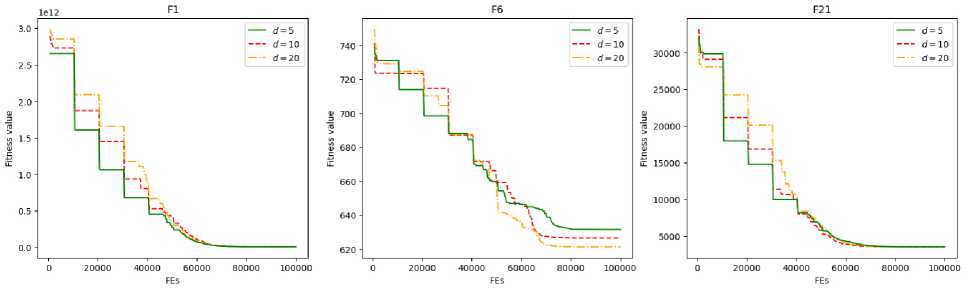
Рис. 4. Графики сходимости алгоритма для разного размера кода для задач размерности 100 (относительно общей популяции)

Fig. 4. Convergence graphs comparison for different code dimensionality on 100D medium-budget problems relative to overall population

Algorithm performance results are summarized in Tables 4–5, where F_i denotes the i -th problem from CEC2022 benchmark. Table 5 additionally provides algorithm comparisons using Wilcoxon rank-sum test with the significance level (significance level α = 0.05). The symbols indicate that the algorithm performed significantly better («+»), worse («–»), or not different («=»). Comparisons are provided between L-AEDE and L-SRTDE, as well as between AEDE and SRTDE.

Table 4

Optimization results and comparison (min)

Problem, D	L-AEDE	L-SRTDE	AEDE	SRTDE
f 1 , 20	1.000e+02	1.986e+02	2.164e+08	3.127e+08
f 6 , 20	6.000e+02	6.000e+02	6.186e+02	6.230e+02
f 21 , 20	2.306e+03	2.312e+03	2.428e+03	2.426e+03
f 25 , 20	2.910e+03	2.906e+03	2.914e+03	2.997e+03
f 1 , 100	4.798e+09	3.896e+09	3.728e+11	6.143e+11
f 6 , 100	6.166e+02	6.158e+02	6.265e+02	6.338e+02
f 21 , 100	2.614e+02	2.731e+02	2.645e+02	2.745e+02
f 25 , 100	3.538e+03	3.538e+03	3.546e+03	3.552e+03
F 5 , 20	1.143e+03	1.136e+03	1.233e+03	1.206e+03
F 11 , 20	2.900e+03	2.900e+03	2.964e+03	2.964e+03

Table 5

Optimization results and comparison (mean)

Problem, D	L-AEDE	L-SRTDE	AEDE	SRTDE
f 1 , 20	2.071e+03	2.756e+02 +	3.365e+08	3.647e+08 -
f 6 , 20	6.000e+02	6.000e+02 =	6.216e+02	6.230e+02 -
f 21 , 20	2.642e+03	2.670e+03 -	2.454e+03	2.451e+03 =
f 25 , 20	2.912e+03	2.908e+03 =	2.967e+03	3.011e+03 -
f 1 , 100	1.379e+10	7.847e+09 +	5.236e+11	6.935e+11 -
f 6 , 100	6.226e+02	6.233e+02 =	6.269e+02	6.339e+02 -

f 21 , 100	2.616e+02	2.623e+02 -	2.831e+02	2.846e+02 =
f 25 , 100	3.666e+03	3.666e+03 =	3.686e+03	3.695e+03 =
F 5 , 20	1.168e+03	1.146e+03 +	1.245e+03	1.239e+03 =
F 11 , 20	2.900e+03	2.900e+03 =	2.967e+03	2.964e+03 =
+ \ – \ =	vs. L-AEDE:	3 \ 2 \ 5	vs. AEDE:	0 \ 5 \ 5

As can be seen from the tables, the population reduction mechanism significantly impacts the convergence speed of the algorithms. Notably, when this mechanism is applied to AEDE, the degradation in performance is less noticeable than for the base method, likely due to the local properties of the subspaces generated by the autoencoder. In configurations without population reduction, AEDE achieved superior results in 50 % of the test cases. However, with population reduction active, L-SRTDE yields more consistently robust performance, especially on problems featuring a difficult to locate global optimum under a constrained evaluation budget (e.g., f 1).

A notable limitation comes from the autoencoder's training on successful solutions, as the resulting latent spaces may cover attraction basins of previously discovered optima, potentially impairing global exploration. The difference in effectiveness remains stable as dimensionality increases, indicating that the proposed method exhibits comparable or reduced sensitivity to the "curse of dimensionality" relative to traditional EAs.

Conclusion

This work proposes an evolutionary algorithm incorporating a dimensionality reduction mechanism based on an autoencoder. The framework is built upon a hybrid search strategy that operates in both the original and latent spaces. This architecture is designed to enhance the efficiency of classical evolutionary algorithms and overcome challenges typical of high-dimensional problems under a tight budget for objective function evaluations. During operation, computational resources are adaptively reallocated, and solutions are exchanged between the search spaces. The presented approach allows for dynamic model training, enabling the identification of promising search regions.

The algorithm was evaluated on a suite of benchmark problems; the obtained results are presented in the form of tables and convergence graphs. Numerical experiments demonstrated that the algorithm is suitable for solving complex black-box optimization problems. These experiments revealed several characteristics of autoencoders in speeding up the search. Several challenges remain for future investigation, including the selection of the neural network's architecture and hyperparameters, as well as the strategy for selecting data to manage global and local convergence.

Acknowledgment. The study was supported by grant No. 24-21-00215 from the Russian Science Foundation,