Examples of quantum computing toolkit: Kronecker product and quantum Fourier transformations in quantum algorithms

Author: Reshetnikov Andrey, Tyatyushkina Olga, Ulyanov Sergey, Tanaka Takayuki, Yamafuji Kazuo
Journal: Сетевое научное издание «Системный анализ в науке и образовании» @journal-sanse
Article in issue: 3, 2017.
Free access
Quantum mechanics requires the operations of quantum computing to be unitary, and makes it important to have general techniques for developing fast quantum algorithms for computing unitary transformations. A quantum routine for computing a generalized Kronecker product is given. Applications for computing the Walsh-Hadamard and quantum Fourier transform is include also re-development of the according network.
Quantum computing, generalized kronecker product, quantum fourier transform
Short address: https://sciup.org/14123273
IDR: 14123273
Примеры инструментария квантовых вычислений: произведение Кронекера и квантовое преобразование Фурье в квантовых алгоритмах
Квантовая механика требует, чтобы операции квантовых вычислений были унитарными, и делает важным иметь общие методы для разработки быстрых квантовых алгоритмов вычисления унитарных преобразований. В работе представлена квантовая подпрограмма для вычисления обобщённого произведения Кронекера. Приложения для вычисления Уолша-Адамара и квантового преобразования Фурье включают в себя также проектирование соответствующей сети.
Text of the scientific article Examples of quantum computing toolkit: Kronecker product and quantum Fourier transformations in quantum algorithms
The efficient implementations of a number of operations for quantum computation include controlled phase adjustment of the amplitudes in a superposition, permutation, approximations of transformations and generalizations of the phase adjustments to block matrix transformations. These operations generalize those used in quantum algorithms. Moreover, the Hadamard transform (H), the phase (Ph), and the CNOT generate the Clifford group. A quantum computation using only operations from this group can be simulated efficiently on a classical computer. The addition of just the Toffoli gate to this group is sufficient to make this group universal. We demonstrate application of this approach to the Benchmarks as Deutsch, Deutsch – Josza, Simon, Shor, and Grover algorithms [1-18].
Physical Principles for Quantum Computation
Here, are the five essential criteria, which we perceive for the physical implementation of quantum computing:
-
1 .Hilbert space control
-
2 .State preparation
-
3 .Low decoherence
-
4 .Controlled unitary transformations
-
5 .State-specific quantum measurements
The first criterion means that the available states must be precisely enumerated, and it must be known how to confine the state vector of the quantum system to this part of Hilbert space. In addition, Hilbert space should be extendable, preferable with a simple tensor-product structure, by adding particles to the system. For example, n spin-1/2 particles have a simple spin Hilbert space of 2 n dimension.
The second criterion . Within this Hilbert space, it must be possible to set the state vector initially to a simple fiducially starting state. A simple example of this, in the spin system, would be to set all the spins in the spin-down state. Frequently this only requires being able to bring the system to sufficiently low temperature that it is in its ground state. This is more difficult in some examples than in others.
The third criterion . The coupling to the environment (i.e., to all the rest of the Hilbert space of the world) should be sufficiently weak that quantum interference in the computational Hilbert space is not spoiled. Given our current understanding of error correction and fault-tolerant quantum computation, and given fairly benign assumptions about the nature of the decoherence (e.g., that it acts independently on each quantum bit) reliable computation is possible if the decoherence time exceeds the switching time by 106 . More clever fault-tolerant techniques may well in making this rather demanding threshold number more relaxed in the future.
The fourth principle. This is the fairly obvious central requirement of quantum computing: it must be possible to subject the computational system to a controlled sequence of precisely defined unitary transformations. The precision requirements are closely related to the decoherence threshold; imprecision of unitary operations is a form of a decoherence. For convenience of programming, it is very desirable that the elementary unitary transformations be implementable as discrete one- and two-qubit operations.
The fifth principle . The readout of a quantum computation, which would consist of some ordinary bit string, is to be the result of a sequence of quantum measurements performed on the computational quantum system. It is very desirable (although not necessary) that these measurements be the textbook projection subsystems of individual quanta. It is essential that these measurements can be made on specific, identified subsystems of the computational state; in the simplest case, this means that it should be possible to do a projection measurement on each qubit individually. If many identical copies of the quantum computer are available, then weaker, ensemble measurements, rather than projection measurements are adequate. It is still necessary that these ensemble measurements be subsystem-specific, though.
Tools for Quantum Computation and Quantum Networks.
To exploit the power of quantum computation and create algorithms of new complexity classes, we need to use building blocks that do not have classical analogs but instead take advantage of quantum parallelism through modifying and mixing amplitudes in superposition. Two sorts of tools have been used effectively in design of quantum algorithms that have been developed so far.
First , transformations that can mixing amplitudes, such as the Walsh-Hadamard and Fourier transforms.
Second , selective adjustment of the phases of certain states that, when combined with a mixing transform, promote amplitude cancellation or amplification. Such phase adjustments form the basis of search algorithms for NP problems.
Here, we discuss efficient implementations of mixing transformations and of relative phase changes that combine amplitude from only a small number of states. The choice of phase and which states to mix depends on a classically efficient computable function f that in general will remain necessarily abstract. We discuss implementations of approximations of transformations, of phase changes, of permutations, and generalizations of the phase change techniques to block matrix transformations. For each of these transformations, we describe the resources in terms of time, number of calls to f , and number of additional qubits needed for the implementation.
We first concern with transformations that change the relative phases of components that make up superposition. Such transformations correspond to acting on the state with a diagonal matrix D . Conversely, because quantum operations are unitary, any operation described by a diagonal matrix will consist of such phase adjustments. Since a global phase change has no physical meaning, so the matrix is only well defined up to multiplication by a constant.
In implementing quantum algorithms it will be useful to have a variety of techniques depending on whether number of bits or coherence time (number of operations) is the main limiting factor. For implementing relative phase changes to components of an n - qubit quantum state several methods can be represented as 2 n x 2 n diagonal matrices D .
If D is decomposable, in that can be written as a tensor product of single qubit rotations, it can be implemented trivially in O ( n ) steps without any additional qubits or function calls.
We describe a sufficient and necessary condition for the decomposability of the matrix D .
N x N unitary matrix, where N is an even
In general form suppose that a unitary matrix U is an number. Then one can always express U in the form
U =
L 1
D
R 0
R 1
NN where the left and right side matrices Lo, Lv, Ro, R, are — x —
unitary matrices and
D =
D 00
D 10
D 01
D 11
For all i e

f 7
, D 00 = D = diag C i, C 2 ..., C
V
, D 01
2 7
—
■ D10 = diag f S , S V
S N
2 7
.
N 1
2 J
, C = cos ^ and St = sin ^ for some angle ^ .
Given any approximation CSD of U , it is possible to find another CSD of U for which the angles ^
are in non-decreasing order and they are contained in the interval [0,900 ]. If one partitions U into four blocks U
NN of the size — x — , then we can obtain U..
2 2 ij
= LDR , for i , j e { 0,1 } . Thus, D . gives the
singular values of U .
Example . The operator D ( diffusion – inversion about average ) in Grover algorithm is
The availability of single quantum systems has fed the interest in quantum networks: A quantum computation is a network of individual quantum systems, where any two of the nodes can interact with each other. Most quantum private communication scheme is networks of two or three nodes. In addition to these information processing and communication related applications, networks avoided crossings in multilevel systems and have been considered in order to study higher dimensional quantum interference effects. Such networks can be experimentally realized by various active (energy-consuming) or passive (energypreserving) components. It is found that transitions do take place and we are able to give them a clear physical interpretation. For active systems the transition is related to quantum and classical, for passive systems to adiabatic and diabatic behavior of the network. The transition phenomenon is clearly reflected in observable quantities and shows a relation to symmetry, which can be of general significance for quantum networks.
In general form the quantum network is represented in Fig. 1.
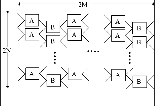
Figure 1: A quantum network where the nodes are connected to their neighbor. The boxes A and B denote the transitions performed at the nodes)
And can be described by a 2 n x 2 n plane rotation matrix P , which is
A
_ А
B 21
B
P =
A
( cosh 0 i sinh 6 А
V— г sinh 6 cosh 6 )
B
A
B
6 cosh ф
V — i sinh ф
i sinh ф а cosh ф ,
B
coth 6 = cosh ф
The form of the matrix P suggests immediately a quantum-network analog. The matrices A and B can be interpreted to describe the evolution of a two-state or two-mode system. The matrix P is then the evolution operator over period in the network of Fig.1. The input of the network are mixed pair-wise according to the transition B , and then the pairs are let to interact with the neighboring ones by applying the shifted set of operations A . By repeating this k times, a 2 n x 2 1 — dimensional network can be constructed. Since P contains all the physical information of the quantum computation, i.e., the phase transitions, we may expect analogous phenomena in the quantum network described by P .
Remark. The physical realization of the quantum network P can be divided into groups. When the angle ф is real, A and B are SU (1,1) - type matrices describing energy - consuming (active) operations. Imaginary ф leads to SU (2) matrices, which correspond to energy - preserving (passive) manipulations of the two modes or two states. Note that A ^ 1 2 when the angle ф ^ ^ , and B ^ I 2 when ф ^ 0 ( 1 2 is the two-dimensional unit matrix). That is, in both of these limits the network decomposes into sets of noninteracting modes. Thus P describes a quantum network where only nearest neighbors interact, and where a single parameter ф determines the relative importance of the interactions, i.e., the network character of the system.
The transitions in the network are determined by the eigenvalues of P . The only problem in diagonalizing P is the relative shift between the set of A and B . This can be solved by the discrete FFT (see below) as ( Fn )^ = exp { i 2 nkk / n}4n = ^ k 14n , because the FFT of the shift matrix ( Sn ) kk = 5 k + 1, k + 5 k , n — X 5 k 0 is diagonal: F nSnFn = D ^ , where ( D o ) kk = ^kk •
The whole network matrix P thus decomposes into
( RA ° 2
( f : ® i 2 )
P = ( F n ® 1 2 ) 0 2 ^
V
K , — 1
)
where ( Kn )H = ( Kn )22 = C ( 0 ) C ( ^ ) + S ( б ) S ( ф ) ю n , C = cosh and S = i sinh and
( k . ) 12 = ( k . ) 21 =— C to S ( 0 ) + C ( 0 ) S ( p ) « - ' .
Example . The usual Mach – Zehnder interferometer (see below) affects the input states by unitary transformation U , which can be formally written as
U m — , = ( F 2 ® 1 1 ) f K 0 ” ^( F 2: ® 1 1 ) ,
V 0 K 1 )
where K = exp { i φ n } is determined by a chosen phase φ . Thus this network-type we consider acts like an n - dimensional interferometer where, instead of one-mode phase shift, two-mode rotations are performed in between the n - dimensional mixers F and F ∗ .
General Structure of Quantum Gates
For this case we use coherent initial classical states and three quantum operators: superposition , entanglement , and interference . These operators are generators of Cliffird group, together with Toffoli gate are universal and can be efficiently realized on classical computer.
Model Description of Three Quantum Operators. Quantum Algorithms are global random algorithms based on the quantum mechanics principles, laws, and quantum effects. In the quantum search, each design variable is represented by a finite linear superposition of classical initial states, with a sequence of elementary unitary steps manipulate the initial quantum state I i (for the input) such that a measurement of the final state of the system yields the correct output. It begins with elementary classical preprocessing, and then it applies the following quantum experiment: starting in an initial superposition of all possible states, it computes a classical function, applies a Quantum Fast Fourier Transform ( QFFT ), and finally performs a measurement. Depending on the outcome it may carry out one more similar quantum experiments, or complete the computation with some classical post-processing. Usually, three principle operators, i.e. linear superposition (coherent states), entanglement , and interference , are used in the quantum search algorithm and briefly described below.
Linear Superposition . Linear superposition is closely related to the familiar mathematical principle of linear combinations of vectors. Quantum systems are described by a wave function ψ that exists in a Hilbert space.
The Hilbert space has a set of states, I φ , that from a basis, and the system is described by a quantum state, ψ = ∑c I φ . The vector ψ is said to be in a linear superposition of the basis states Iφ , and in i the general case, the coefficients c may be complex. Use is made here of the Dirac bracket notation, were the ket I ⋅ is analogous to a column vector, and the bra ⋅ I is analogous to the complex conjugate transpose of the ket. In quantum mechanics the Hilbert space and its basis have a physical interpretation, and this leads directly to perhaps the most counterintuitive aspect of the theory. The counter intuition is this (at the microscopic level), the state of the system is described by the wave function ψ , that is, as a linear superposition of all basis states (i.e. in some sense the system is in all basis states at ones). However, at the macroscopic or classical level the system can be in only a single basis state. For example, at the quantum level an electron can be in a superposition of many different energies; however, in the classical realm this obviously cannot be.
Remark: Coherence and Decoherence. Coherence and decoherence are closely related to the idea of linear superposition. A quantum system is said to be coherent if it is in a linear superposition of its basis states. A result of quantum mechanics is that if a system is in a linear superposition of states interacts in any way with its environment the superposition is destroyed. This loss of coherence is called decoherence and is governed by the wave function ψ . The coefficients c are called probability amplitudes, and Ic I 2 gives the probability of ψ collapsing into state I φ if it is decoherence. Note that the wave function ψ describes a real physical system that must collapse to exactly one basis state. Therefore, the probabilities governed by the amplitudes c must sum to unity. This necessary constraint is expressed as the unitary condition ∑Ic I = 1 . In the Dirac notation, the probability that a quantum state ψ will collapse into an eigenstate i
I φ is written |( φ i ψ }| and is analogous to the dot product (projection) of two vectors.
Consider, for example, a discrete physical variable, called spin. The simplest spin system is a two-state system, called a spin-1/2 system, whose basis states are usually represented as |T^ (spin up) and |T^ (spin down). In this simple system the wave function у is a distribution over two values (up and down) and a coherent state | y ) is a linear superposition of Ту and Ty .
Example . One such state might be | у ^ = —y=|T^ + —^=|T^ . As long as a system maintains its quantum coherence it cannot be said to be either spin up or spin down. It is in some sense both at ones. Classically, of course, it must be one or the other, and when this system decoherence the results is, for example, the | Т state with probability |^Т| у ^| = ( 2^ ) 2 = 0.8 . A simple two-state quantum system, such that as the spin-1/2 system just introduced, is used as the basis unit of quantum computation. Such a system is referred to as a quantum bit or qubit , renaming the two states 0 and 1 it is easy to see why this is so.
Remark : The Operators . Operators on a Hilbert space describe how one wave function is changed into another. Here they will be denoted by a capital letter with a hat, such as A , and they may be represented as matrices acting on vectors. Using operators, an eigenvalue equation can be written A|фф = а,|ф ) , where at is the eigenvalue. The solutions фф to such an equation are called eigenstates and can be used to construct the basis of a Hilbert space. In the quantum formalism, all properties are represented as operators whose eigenstates are the basis for the Hilbert space associated with that property and whose eigenvalues are the quantum allowed values for that property. It is important to note that operators in quantum mechanics must be linear operators and further that they must be unitary so that A * A = ЛЛ * = 7 , where 7 is the identity operator, and A * is the complex conjugate transpose, or joint, of LA .
Interference. Interference is a familiar wave phenomenon. Wave peaks that are in phase interfere constructively (magnify each other’s amplitude) while those that are out of phase interfere destructively (decrease or eliminate each other’s amplitude). This is a phenomenon common to all kinds of wave mechanics from water waves to optics. The well known double slit experiment demonstrates empirically that at the quantum level interference also applies to the probability waves of quantum mechanics.
Example. As a simple example, suppose that the wave function described in (3) is represented in vector
form as
f 2 )
^7
and suppose that it is operated upon by an operator H
(Hadamard transform)
w
7 1 f 1
described by the following matrix, H = —;= _
2 I1
- 1 . )
and therefore now
;= I Th —:= IT). Notice that the amplitude of the IТ) state has increased while 10 10
the amplitude of the |T^ state has decreased .
This is due to the wave function interfering with itself through the action of the operator – the different parts of wave function interfere constructively or destructively according to their phases just like any other kind of wave.
Entanglement. Entanglement is the potential for quantum states to exhibit correlation that cannot be accounted for classically. From a computational standpoint, entanglement seems intuitive enough (it is simply the fact that correlation can exist between different qubits) for example if one qubit is in the 1 state, another will be in the 1 state. What makes it so powerful is the fact that since quantum states exist as superpositions, these correlation somehow exist in superposition as well. When the superposition is destroyed, the proper correlation is somehow communicated between the qubits, and it is this ‘communication’ that is the crux of entanglement. Mathematically, entanglement may be described using the density matrix formalism. The density matrix p of a quantum state |и) is defined as p = |k)k|• For example, the quantum state |^) = -/= 100^ + —j= |01) appears in a vector form as
f1 ]
|0 J and it may also be represented as density matrix
( 1 I 0
,
while the state | И = ^= 100) + ~/= 111), is represented as
;
I :
0 ' 0 1
and the state IZ = 100) +—;= 101) +— as
|
f 1 |
1 |
0 |
1 ) |
|
|
1 |
1 |
0 |
1 |
|
|
P z = K X Z = 3 |
0 |
0 |
0 |
0 |
|
1 1 |
1 |
0 |
1 J |
where the matrices and vectors are indexed by the state labels 00,^11. Now, notice that p can be factorized as
1 (( 1 0 )
®
( 1 1 ))
I1 1
, where ® is a normal tensor product. On the other hand,
P v
cannot be factorized. States that cannot be factorized are said to be entangled, while those that can be factorized are not. Notice that p can be partially factorized two different ways, one of which is
(
p = V3


0 1T0 0
0 0
0 0J,
(the other involves above equation and a different remainder); however, in both cases the factorization is not complete. Therefore, p is also entangled, but not to the same degree as p (because p can be partially factorized but p cannot). Thus there are different degrees of entanglement.
Remark. It is interesting to note from a computational standpoint that quantum states that are superpositions of only basis states that are maximally far apart in terms of Hamming distance are those states with the greatest entanglement. For example, p is a superposition of only the states 100) and 111) , which have a maximum Hamming spread, and therefore p is maximally entangled. Finally, it should be mentioned that while interference is a quantum property that has a classical cousin, entanglement is a completely quantum phenomenon for which is no classical analog.
Quantum Networks . Quantum networks are one of the several models of quantum computation. Others include quantum Turing machines, and quantum cellular automata. In the quantum networks model, each unitary operator is modeled as a quantum logic gate that affects one, two or more qubits. Schematically this is represented as a set of quantum ‘wires’ entering and leaving quantum gates, reminiscent of classical logic networks.
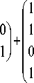
For example, Fig. 2 shows a network that operates on three qubits, which are represented as lines.
By convention the logic flows from left to right. The gates are represented as boxes and labeled with the operators that they represent. A dot on a quantum “wire” represents a conditional upon that qubit.
Therefore, in the quantum network shown in Fig. 2 an operator A represents a single qubit quantum gate, B and C represent 2-qubit quantum gates, and D represents a conditional 3-qubit gate. Suppose that A is an operator that flips the state of qubit, B is an operator that exchanges the states of two qubits if they are equal, and DD is an operator that exchanges the states of two qubits if a third qubit in the | 1^> state. When three qubits “enter” the quantum logic network, the one labeled q first has its state flipped; then q and q exchange states, q and q have their states flipped if they are equal, and finally q and q exchange states if q 1 is in the state 1 . Of course, if the qubits “entering” the logic array did not exist in a superposition states, this would be no different than a classical logic sequence. However, the qubits do exist in a superposition of states; therefore, these gates or operations are applied to all the states in the superposition simultaneously, resulting in what has been called quantum parallelism. Recall that the quantum logic gate arrays are simply a schematic way to represent the time evolution of a quantum system. They are not meant to imply that quantum computation can be physically realized in a manner similar to classical logic networks. Alternatively, the network could be represented as a product of quantum operators. Since operators are applied right to left, the network of Fig. 2 would be represented as the operator product DDCBBA in what follows, both the network and the product of operator representations will be used.
Interference and Quantum Parallelism . Because of the entanglement or quantum correlation between the n quantum particles, the state of the system cannot be specified simply describing the state of each of the n particles. Instead, the state of n quantum bits is a complicated superposition of all 2 n basis states, so 2 n complex coefficients are needed in order to describe it. This exponentially of a Hilbert space is a crucial ingredient in quantum computation. To gain more understanding of advantages of the exponentiallity of the 1
space, consider the following superposition on n quantum bits, ^= ^|i^,z2 ,•••,z„ ^. This is a uniform i1 ,i2 <",in =0
superposition of all possible basis states of n qubits. If we now apply the unitary operation U which computes f for this state, we will get, simply from linearity of quantum mechanics: 11
"p 21 ii,i2, ^ ,in) ^ "p 21 f ( i 1 , i 2 ,'"» in )). Applying the unitary operator Uf once, computes f
Hi i 2 , ^ , i n = 0 i 1 , i 2 ,"', i n = 0
simultaneously on all the 2 n possible inputs i , which is an enormous power of parallelism. It is tempting to think that exponential parallelism implies exponential computational power, but this is not the case. In fact, classical computations can be viewed as having exponential parallelism as well. The problem lies in the question of how to extract the exponential information out of the system .
In quantum computation, in order to extract quantum information one has to observe the system. The measurement process causes the famous collapse of the wave function. In nutshell, this means that after the measurement the state is projected to only one of the exponentially many possible states, so that the exponential amount of information, which has been computed, is completely lost. In order to gain advantage of exponential parallelism, one needs a combine it with another quantum feature, known as interference. Interference allows the exponentially many computations done in parallel to cancel each other, just like destructive interference of waves or light. The goal is to arrange the cancelation such that only the computations, which we are interested in remain, and all the rest canceled out.
The combination of exponential parallelism and interference is what makes quantum computations powerful and plays an important role in quantum algorithms. The Fourier transform indeed manifests interference and exponentiallity .
Logic Gates and Quantum Computations. In classical computations and in digital electronics, one deals with sequences of elementary operations (operations such as AND, OR and NOT). These sequences are used to manipulate an array of classical bits. The operations are elementary in the sense that they act on only of few bits (one or two) at a time. We will (some times) refer to sequences as products and to operations as operators, matrices, instructions, steps and gaits. Further more we will introduce the sequences of elementary operations as basis of quantum computation. In quantum computation one also deals with sequence of elementary operations - SEO (with operations such as controlled-NOT’s and qubit rotations), but for manipulating qubits instead of classical bits. Quantum sequences of elementary operations are often represented graphically by qubit circuits. In quantum computation, one often knows the unitary operator U that describes the evolution of an array of qubits. One must then find a way to reduce U into the sequence of elementary operations. The algorithm can be applied to any unitary operator U . It is useful to define certain unitary operator UN for all NB e { 1,2,3, •” } , where UNg is a 2 N B x 2 N B matrix and NB is the number of bits. Some U are known to be expressible as a sequence of elementary operations whose lengths (i.e. whose number of elementary operations) is a polynomial in N B . Two examples are the N B bit Hadamard transform (HT) matrix and the N B bit discrete Fourier transform (DFT) matrix. The HT matrix is known to be expressible as a sequence of elementary operations of lengths Order ( N ). The DFT matrix is known to be expressible (using the Fast Fourier Transform (FFT) algorithm) as a sequence of elementary operations of lengths Order ( N 2 ). Presented algorithm achieves both of these sequences of elementary operations (SEO)
lengths as benchmarks. Even better the SEO often called the “Quantum FFT algorithm” is exactly reproduced by this algorithm.
Previously another algorithms have described for reducing a unitary operator into SEO, and their algorithm can be applied to any unitary operator U . However, it is very unlikely that their algorithm can be efficient in producing short SEO’s unless farther optimizations are added to it. And such optimizations, if they exist, have not been specified by anyone.
Benchmarks of Quantum Gates for Quantum Algorithm’s Design
We represent the general approach to design of quantum gates for quantum algorithms. The results of this approach are described in Table 1.
Table 1: Benchmarks of Quantum Gates for Quantum Algorithms
|
Name |
Al g orithm |
Gate : Symbolic Form |
||||
|
Detsch — Jozsa |
m = 1; Int = n H ® I ; k = 1; h = 0 |
|||||
|
entanglement ( n H ® I ) • UF • ( n + 1 H ) int erference sup erposition |
||||||
|
Simon |
m = n ; Int = n H ® n H ; k = O ( n ) ; h = 0 |
|||||
|
entanglement ( n H ® n H ) • UF • ( 2 n H ) int erference sup erposition |
||||||
|
Shor |
m = n ; Int = QFT„ ® n H ; k = O ( n 2 ) ; h = 0 |
|||||
|
entanglement ( QFT n ® n H ) • U f ■ ( 2 n H ) int erference sup erposition |
||||||
|
Grover |
m = n ; Int = Dn ® I; k = 1; h = O ( 2 n/2 ) |
|||||
|
entanglement | ( D n ® 1 ) • U f | int erference |
h • ( n + 1 H ) sup erposition |
|||||
Using this approach the methodology of quantum algorithm simulation on classical computer is developed. The concrete result of simulation Deutsch – Jozsa, Simon, Shor and Grover algorithms are described in main text. The results of this approach in Table 1 are described.
Any relations with Walsh-Hadamard Transformation. The Hadamard (rotation) transformation is one of the simplest and most common fault-tolerant operations. The gate equation is = — — H(t)U(t), which at h is subject to initial condition U(0) = I and target condition U(T) = U0. Here U0 is the matrix of the desired gate.
The wave function | ^ ( t )) is related to the evolution operator U ( t ) and the initial wave function | ^ ( 0 )} by | ^ ( t )) = U ( t ) ^ ( 0 )) . We choose the various quantum gates from physics point of view in such a way that they can be described by simple Hamiltonians The gates correspond to the unitary operation
( W ^ R ^ H ) effected by the
Hamiltonian H
П 1/
2 2 °
X —
°z ) + 1 acting for one unit at time.
1 ( 1
Similarly the gate U = —j= y 2
I-1
generated by the Hamiltonian Hy = - “°\ acting for one unit of
time. The solutions of corresponding Schrodinger equations with these types of Hamiltonians are described the evolution with coherence states (with minimum of uncertainty ), i.e., the gates are robustness and fault-tolerant.
Remark : Physical and Geometrical Interpretations of Walsh-Hadamard Transformations. It is natural to think of quantum computations as mutiparticle processes. Just as classical computations are processes involving several “particles” or bits. It turns out that viewed quantum computation as multiparticle interferometry leads to a simple and unifying picture of known quantum algorithms. In this language quantum computation are basically multiparticle interferometers with phase shift that result from operations of some quantum logic gates. To illustrate this point consider, for example, a Mach-Zehndler interferometer in Fig. 3a.
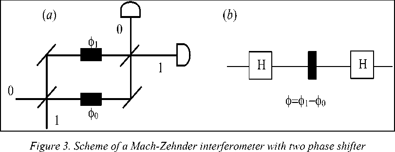
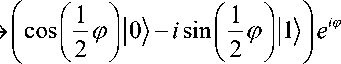
The interference pattern depends on the difference between the phase shifts in different arms of the interferometer. (a) The corresponding quantum network representation. (b) mirror which directs the particle to one of the two detectors. Along each path between the two half-silvered mirrors is a phase shifter. If the lower path is labelled as state 0 and the upper one as state 1 , then the state of the particle in between the half-silvered mirrors and after passing through the phase shifters is a superposition of the type Principle Description of Mach-Zehnder Interferometer. A particle, say a photon, impinges on a half-silvered mirror, and, with some probability amplitudes, propagates via two different paths to another half-silvered —j= ( 0^ + e‘(ф1 ф0)| 1), where ф0 and ф; are the setting of the two phase shifters. The phase shifters in the two paths can be tuned to effect any described relative phase shift ф = фх — ф and to direct the particle with probabilities — (1
+ cos
ф)and 1 (1
— cos ф ) , respectively, to detectors “0” and “1”. The second half-
silvered mirror effectively erases all information about the path taken by the particle (path 0 or path 1 ) which is essential for observing quantum interference in the experiment.
Physical Interpretation of Walsh-Hadamard Transformation. According to this description let us now rephrase the experiment in terms of quantum logic gates. We can identify the half-silvered mirrors with single-qubit Walsh-Hadamard transform. We view the phase shifter as a single-qubit gate (see Fig. 3, b). The phase shift can be “computed” with the help of an auxiliary qubit (or a set of qubits) in a prescribed state u and some controlled- U (c- U ) transformation where U| u^ = eiф | u) (see Fig. 3, b). Here, the controlled - U transformation depends on the logical value of the control qubit; for example, we can apply the identity transformation to the auxiliary qubits (i.e. do nothing) when the control qubit is in state 0 and apply a prescribed U when the control qubit is in state 1 . The controlled - U operation must be followed by a transformation which brings all computational paths together, like the second half-silvered mirror in the Mach-Zehnder interferometer. This last step is essential to enable the interference of different computational paths to occur – for example, by applying a Walsh-Hadamard transformation. In this example, we obtain the following sequence of transformations on the two qubits:
0 u
>
^(l 0+ e *
11) )l u
- ^ (10) +11} )l u} c —U
H
u
The state of the auxiliary register u , being an eigenstate of U , is not altered along this network, but its eigenvalue е1ф is “kicked back” in front of the 1 component in the first qubit. This sequence is the exact simulation of the Mach-Zehnder interferometer and the kernel of quantum algorithms.
Geometrical Interpretation of Walsh-Hadamard Transformation. The Hilbert space of one qubit (i.e. a two-dimensional Hilbert space) equipped with a standard basis denoted by В = ( 0^, 11) The dual basis of В denoted by (0'),|1')) is defined by 10'^ = -^(0)+ Ц , |1'^ = -^=(0)- Ц . Thus H2 = I and H interchange the standard and dual bases. In terms of real geometry, the dual basis lies on the 45 0 lines between the orthogonal directions 0 and 1 (see, Fig. 4) and H is the transformation given by reflection in a line at angle — n to the |0) direction. Thus the eigenvectors of H (parallel and perpendicular to the 8
mirror line) are cos| — 0^ ± sin
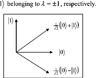
Figure 4. The relations between standard and dual bases
1 8 J '
If x = ( Xy ,.. xn ) and y = ( y t,. yn ) are in В n , then by the inner product between two bit strings x and y , we mean the inner product modulo 2, that is: ( x , y ) = x • y = ( x^y Ф ■ • • Ф xny n ) . This value can also be viewed as the parity of a subset of the bit string y 1 ■ • yn (the parity of the number of places where x and y both have a bit value of 1).This subset is described by the characteristic vector x and its size equals the Hamming weight || x || of the bit string x , • xn . The parity basis is the now familiar result of the one bit Hadamard gate (see, Fig. 4).
The Hadamard transformation of a sequence of bits yx • • yn and the inner product function are closely related to each other: for any y e{0,1}n it holds that H® |y) = .— ^(— 1)(x,y)| x) • 42n xe{0,1}}
Because H is its own inverse, we can apply again a sequence of n Hadamard transforms on the these states and thus obtain the original bit string y1 • y again: H® ( .— ^(—1)(x,y)|x)) = Iy\ . The above
V2n xe{0,1}} leads to the observation that if we want to know the string y • y , it is sufficient to have a superposition with phase values of the form (—1)(x,y), for every x e {0,1}n . This is a well-known result in quantum computation and has been used several to underline the differences between quantum and classical information processing.
The scalar product modulo 2 as ( x , y ) = x • y = ( x x л y^ ) ф • Ф ( xn л yn ) is the XOR of the bitwise AND of the two strings x and y , and equivalent to performing a one-qubit Hadamard transform on each of the n qubits individually.
Applications of Walsh-Hadamard Transformation in Mixing Operations . For effective quantum algorithms, we also need to be able to effective mix amplitudes in a superpositions so as to increase the change of a desired reading being made. One way to achieve this mixing is to combine an efficiently implementable diagonal matrix with a decomposable mixing matrix. For instance, a number of existing algorithms make use of mixing matrices of the form HDH where D is a diagonal matrix and H is the
Walsh-Hadamard transformation given by H = W
. We have described below efficient
implementations for certain diagonal matrices that can be combined with the Walsh-Hadamard transformation or other mixing matrices to achieve desireable amplitude interference.
Remark. More general form of Walsh-Hadamard transform is the n-bit Sylvester-Hadamard matrix is defined by
H 1
|
2 x 2 |
0 |
1 |
|
0 |
1 |
1 |
|
1 |
1 |
— 1 |
; H 2
|
4 x 4 |
00 |
01 |
10 |
11 |
|
00 |
1 |
1 |
1 |
1 |
|
01 |
1 |
— 1 |
— 1 |
— 1 |
|
10 |
1 |
1 |
— 1 |
— 1 |
|
11 |
1 |
— 1 |
— 1 |
— 1 |
; H r + i = H i ® H r ; H, 2 = nl „ .
The desired H gate acts on a quantum register by sending each qubit individually into a separate H gate. The unitary transformation induced by an Hn is given by the formula Hn = ®n H. If n > 1 then a nice recursive definition is defined as
H n = H 1 ® H n - 1
н —
V1 n - 1
H
—
X
n - 1
H
n - 1 7
Simple Operations of Hadamard Transform with Simple gates. Let us see what an H gate does to
X , Y , and Z
HXH *
1 ( 1
Y1
—
—'J
( 1 0 )
(o -J= Z ; HZH
1 ( 1
i1
HYH *
1 ( 1 1 Y— 11 )
—
1 7[
1 y 1
—
u
—
( 0 1 J
[1 0 7
( о 1 )
■
[
—
1 0 7
— Y .
Therefore, applying H bitwise will switch all the XS and all the Z ' s , and give a factor of -1 for each Y . This is a valid fault-tolerant operation.
Thus, the Hadamard gate implements the Hadamard transform ; it is the single qubit gate H performing the unitary transformation (see, Fig. 5)
1 ( 1
H = W = .
2 1
— 1 1 )
^ | x ^ ^ H ^ ( — 1 ) x | x ) +1 1 — x)
Figure 5: The Hadamard gate representation. The diagram on the right provides a schematic representation of the gate H acting on qubit in state | x) , with x = 0,1
Consider the following unitary transformation (and associated gate):
P =
[ 0
—
и
^ (11) ^ P ^ (—11)
If a qubit is set to 0 nothing happens, but if is set to 1 the amplitudes is multiplied by –1. This gate “encodes” the value of the qubit into the sign of the amplitude.
Another same common bitwise operation is the i phase: P =
0 J i 7
On the basic operations X , Y ,
and Z it acts as follows:
P X P *
T1 о Y о
- i 1
T 0 - i 1
к0 i Л
1 0J
P Y P *
к i 0
T 1
к0
= iY ; P Z P *
J
0IT0 iJ iJk1 0 J
T 0
к i
T 1
к 0
0 n 0 1
i JV 0 i J
= iX .
( 1 J к 0 1 J
= Z ;
This switches X and Y , but with extra factors of i , so there must be a multiple of 4 X S and Y S for this to be a valid operation. Note that a factor of i appears generically in any operation that switches Y with X or Z , because Y 2 = - 1 , while X 2 = Z 2 =+ 1 . These operations actually permute Pauli matrices: ax = X , a7 = Z , and G Y = iY . The most general single qubit operation can be viewed as a rotation of the Bloch sphere permuting the three coordinate axes.
Remark. The one-qubit operations correspond to the six automorphisms of the group D 4 of products of I, X, Y, and Z (or direct product of copies of D4 for multiple-qubit gates) given by {l, H, P, Q = P* HP *, T = PQ*, T 2 }. So all one-qubit operations are covered. Given any such automorphism, we first substitute iY for Y to get the actual transformation. For instance, consider the cyclic transformation T = X A iY A Z A X . Since Z A X , 10) A
( 0) +|1) ) . Also, X A iY ,
so
^Y ( 0 + 1) ) =
—
(| 0) -1 1) ) . Thus, the matrix for T is T = —:= 12 1' , 12 (1
1 i J
.
We can perform a similar procedure to determine the matrix corresponding to a multiple-qubit transformation.
Example . We can make a copy of entering qubit. The superposition is now ^=(1 00) + 111) ) , i-e-entangled state. If we let the first bit go through the Hadamard gate and do nothing to the second one, the result becomes:
( H ® I ) | 1 (100) + 111) ) | = 1 ( 00) + 110) ) + 1 (101) - 111) )
Each vector has equal norm so we will observe, after measuring, each vector with probability , and in particular the firat bit will be perfectly random. Now let us see what happens if we also make the copy bit go through a Hadamard gate. Will it affect the randomness of the output?
Controlled Two - Bit Gates . The two-bit gates of the network correspond to controlled phase shift .
These are
represented in the canonical basis В = { 00), |01),|10),|11) } by the unitary operator
U =
T 0
к 0
- 0
, generated by the Hamiltonian H = nP^ i ® ^ ^ y, where i and j designate the two
qubits on which the gate acts and P ^ = — ( 1 + r r z )
is the projector on state 1 . In this case a state i , j
|
( H ® H ) | (1 00) + 11) ) к V2. ,ZJ |
-, 1(( 0+11 M 0) +11 )) +, 1 ( 0 11 M 0 11 ) 2 23 2 23 |
|
= 1 (100 +И ) |
Randomness of the first bit remains intact.
picks up a phase n if and only if (iff) both qubits are in state Ц . Variants on this gate can be obtained by replacing either or both of the projectors with P in the definition of the Hamiltonian.
The conditional phase shift is the two-bit gate (see, Fig. 6)
|
1 0 0 0 x—- P ( Ф ) = ° 1 ° ° о 0 0 10 . l0 0 0 еф J y |
■ eM| x)\y) |
Figure 6. The two-bit conditional phase shift gate. The matrix written in the basis
В = { 00), 101), 110), 111) } .The diagram on the right shows the structure of the gate
Controlled Two - Qubit Gates . To see how such unitary operators may be constructed from a few elementary ones we must also consider the controlled-NOT (or XOR ) gate. Just as any classical computation can be expressed as a sequence of one- and two-bit operations (e.g., NOT and AND gates), any quantum computation can be expressed as a sequence of one- and two-qubit quantum gates, i.e., unitary operations acting on one or two qubits at a time (see, Fig. 7).
A
в e л)
Figure 7. Quantum circuit diagram for an XOR gate. The lower bit B is flipped whenever the upper bit
A is set
The standard two-qubit is the controlled-NOT or XOR gate, which flips its second (or “target”) input if its first (“control”) input is |1) and does nothing if the first input is 10) . In other words its interchanges 110)
and |11) while leaving |00) and |01) unchanged. Writing the two-particle basis states as the vectors
( 1 0 0 0 A
|
U xOr = CNOT = |
0 |
1 |
0 |
0 |
|
0 |
0 |
0 |
1 |
|
|
i 0 |
0 |
1 |
0 j |
|
( 1 |
0 |
. CNOT |
|
: 0 |
NOT |
|
|
l |
J |
|
00) |
^ |
00) |
||
|
01 |
^ |
01 |
||
|
10) |
^ |
11) |
||
|
11 |
^ |
10) |
The XOR gate is a prototype interaction between two quantum particles (systems), and illustrate several key features of quantum information, in particular the impossibility of “cloning” an unknown quantum state, and the way interaction produces entanglement. Here the first particle acts as a conditional gate to flip the state of the second particle. It is easy to check that the state of the second particle corresponds to the action of the XOR gate. The quantum circuit for the XOR gate is illustrated in Fig. 8. This circuit is equivalent to the elementary instruction: if (x) = 1) then (| y) = NOT y)), which may be thought of as example of quantum computer code.
|
( 1 0 0 0 ) |
||
|
1 x) |
||
|
0100 |
||
|
CNOT = |
^ |
|
|
0001 |
W |
|
|
v 0 0 10 , |
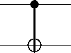

Figure 8. Quantum circuit diagram for an CNOT (XOR) gate. The lower bit y is flipped whenever the upper bit x is set
Remark . The quantum controlled-NOT gate is not a universal quantum gate but a universal quantum gate can be constructed by a combination of the controlled-NOT and simple unitary operations on a single qubit. This means that the XOR gate, together with the set of one-bit gates, from a universal set of primitives for quantum computation; that is, any quantum computation can be performed using just this set of gates without an undue increase in the number of gates used. Unlike one-qubit gates, two-qubit gates are difficult to realize in the laboratory, because they require two separate quantum information carries to be brought into strong and controlled interaction (see below).
If the CNOT (XOR) is applied to Boolean data in which the second qubit is 0 and the first is 0 or 1 (see also, Fig. 8) the effect is to leave the first qubit unchanged while the second become a copy of it: UCNOT I x,0 = | x , x ) for x = 0 or 1. One might suppose that the CNOT operation could also be used to copy superpositions, such as | ^ ) = a\ 0) + в 1, so that U cnот | У- 0 would yield | ^ , ^ ), but this is not so. The unitary of quantum evolution requires that the superposition of input states evolve to a corresponding superposition of outputs. Thus the result of applying UCNOT to | ^ ,0) must be a | 00) + в 11), an entangled state in which neither output qubit alone has definite state. If one of the entangled output qubit is lost (e.g., discarded, or allowed to escape into the environment), the other thenceforth behaves as if it had acquired a random classical value 0 (with probability | a |2 ) or 1 (with probability | в |2). Unless the lost output is brought back into play, all record of the original superposition | ^ ) will have been lost. This behavior is characteristic not only of the CNOT gate but of unitary interactions generally: their typical effect is to map most non-entangled initial states of the interacting systems into entangled final states, which from the viewpoint of either system alone causes an unpredictable disturbance.
Remark. The classical controlled - NOT gate is a reversible logic gate operating on the two bits 8 and 82; 81 is called the control bit and 82 - the target bit. The value of 82 is negated if 81 =1, otherwise 82 is left unchanged (in both cases the control bit 81 remains unchanged). The quantum controlled - NOT gate C 12 is the unitary operation on two qubits, i.e. state in H2, which in a chosen orthonormal basis { 0),Ц} reproduced the controlled - NOT operation: 81)82)—C12 >181)81 © 8 ) , where © denotes addition modulo 2. Here and in the following the first subscript of C always refers to the control bit and the second to the target bit. Thus, for example, C21 denotes the unitary operation defined by I 81 ) I 8 2 ) ^ I 81 © 8 2 )1 8 2 ) .
The properties of controlled – NOT gate . Let us specify any interesting properties of the quantum controlled – NOT gate. The CNOT gate is the idealized discrete operation for producing entangled states.
The quantum controlled-NOT gate tra nsforms superpositions into
Quantum entanglement ,
V
C 12: ( a |0) + b\ 1 ) ^®^ a\ 0|0)) + b |1)|1)
quantum entanglement
As Fig. 9 indicates, a particular product-state input to the gate as shown, using two states from non-orthogonal bases (related by a Hadamard transform), produces at the output the non-product state: ( 01) -110)), a state equivalent to EPR –Bohm pair.
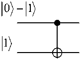
EPR-Bohm pair: 101) -110)
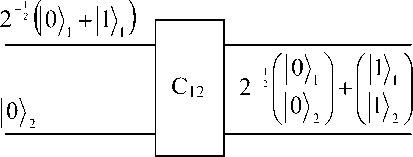
Figure 9. CNOT produces perfectly entangled quantum states from unetangled ones (a); The CNOT gate applied to two qubits. The right hand state entangled; it is not possible to associate a definite state with one qubit independent of the other, as is the case for the left hand side. The reversibility of the gate means that it can be run left to right or right to left (b)
Thus it acts as “the measurement gates” because if the target bit f 2 is initially in state |0) then this bit is in effect an apparatus that performs a perfectly accurate non-perturbing (quantum non-demolition (QND) measurement type) measurement of f. This is illustrated in Fig. 10: if the object is to measure state of the upper qubit (that is , whether it is in the 0 state or the 1 state ), we may CNOT it with a second bit started in the 0 state; then a measurement of the second bit will reveal the desired outcome.
|
0 or 1 0 |
> |
M |
0 or 1 |
|
|
—1 1 |
||||
|
0 or 1 |
||||
Figure 10. CNOT functions as an ideal non-demolition measurement apparatus for a qubit.
This may not appear to be much of a advantage over measuring the first qubit directly. However, it has the feature of being a “non-demolition” measurement in which the original quantum state remains in existence after the measurement. It only remains undistributed if it started in the 0 or the 1 state; if it started in a superposition, then the state is “collapsed” by the measurement.
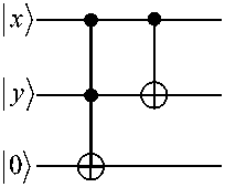
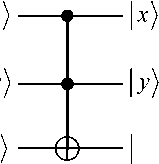
Example. To appreciate the real power of the non-demolition capability of the CNOT gate, consider the simple quantum circuit of Fig. 11.
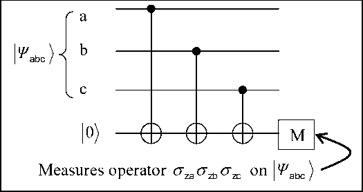
Figure 11. A circuit of CNOTs can be used to do a non-demolition measurement of the three-particle operator shown
The effect of the three successive CNOTs followed by a measurement of the target qubit is to accomplish a highly non-trivial non-demolition measurement of the three-particle Hermitian operator q_gzVgzc . Previous discussions of such three-particle operators always assumed that it would necessarily be done in a “demolishing” fashion where each of the one-particle operators were measured separately. This property forms the basis of the use of the CNOT gate in the implementation of error correction and hence in fault-tolerant quantum computation.
This transformation of superpositions into entanglements can be reversed by applying the same controlled-NOT operation again. If we define a conjugate qubit basis by |0 '^ = —^( 0 ) + Ц and
11'} = -/= ( 0 ) -1 , then it is easy to show that when both input qubits are considered in the conjugate basis, then the effective gate action is an CNOT but with the source and target bits reversed. Hence it can be used to implement the Bell measurement on the two bits by disentangling the Bell states.
For the four Bell states we get for product states disentangled disentangled
- J. (10)10) ± 1010 )=^ (10) ± io )l 0); C 12^ (10)10 ±1110) )=^ (10) ±1 1 )l 0.
Thus the Bell measurement on the two qubits is reduced to the simple sequence of two independent two dimensional measurements: in the basis { 0^, 11} for the control qubit and in the basis —( 0^ ± 11)) for the target qubit. The realization of the Bell measurement is the main obstacle in the practical implementation of quantum teleportation and the dense quantum coding. If just the target bit is represented in the conjugate
|
basis, |
then the |
|
< 10 0 |
|
|
010 |
|
|
U = |
|
|
001 |
|
|
v 0 0 0 |
action of the CNOT is completely symmetric on the two qubits, having the form
0 )
This “phase-shift” form of the gate (controlled-Rotation - CROT) is the one which
- 1)
has been discussed in the cavity quantum-electrodynamic implementation of a two-bit quantum gate by
Turchette, 1995.
The XOR gate allows us to move information around as illustrated in Fig. 12.
|
A |
B |
||
|
C I2 C 2I C I2 ИИ = ИИ |
|||
|
B |
A |
Figure 12. Circuit for swapping a pair of bits
Quantum state swapping can be achieved by cascading three quantum controlled-NOT gates for arbitrary states | ^ and | ^ .
Remark : The quantum controlled-NOT gate is not a universal gate, however, the universal quantum gate can be constructed by a simple extension of the controlled-NOT gate to the controlled-controlled-NOT gate combined with simple unitary operations on a single qubit (see Theorem 1 ).
It is straightforward to show that the CNOT gate induces the following transformation:
|
X 0 I oooo > X 0 X |
Z ® I CN OO > Z 0 1 |
|
I 0 X CN OT > I ® X |
1 0 Z o N oo > z 0 z |
It is easy to see here how amplitudes are copied forwards and phases are copied backwards. For two arbitrary unitary transformations U 1 and U 2 , the “conditional” transformation |0^0| ® Ux + |1}(1| ® U 2 is also unitary. The CNOT gate can defined by
CN0 t = |0)(0| ® I +11)<1| ® X .
The transformation CNOT is unitary since CNOT * = CNOT and CNOT • CNOT = I . The CNOT gate cannot be decomposed into tensor product of two single-bit transformations. A CNOT-operation can be performed in an ion trap by a sequence of three operations: Controlled-ROT Gate, Controlled-SWAP Gate, and Basis Transformations .
Another types of controlled - U gates can be described as in Table 2.
Table 2. Typical controlled - U gates and Its Matrix Representation Forms
|
Title of Operations |
Matrix Presentation Forms |
|
|
CNOT |
( 1 0 0 0 ^ 0 10 0 0 0 0 1 v 0 0 10 J |
|
|
CROT |
1 0 0 0 ^ 0 10 0 0 0 10 0 0 0 - 1 J |
|
|
SWAP |
( 1 0 0 0 ^ 0 0 10 0 10 0 v 0 0 0 1 J |
|
Using the operations from the Table 2 it is possible defined the new operations as in Table 3.
In general form this gate can be written as the unitary transformation in matrix form as in Fig. 13.
Г 1 0
R x У ) =
( 0 0
0 0 ^
0 0
cos(f ) i sin (y )
i sin ( y ) cos ( y )v

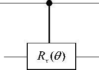
Table 3. Relations between the Operations CROT and SWAP
|
Title of Operations |
Re presentation Forms |
|
CROT ( x , y ) = |
SWAP ( y , x ) * CROT ( x , y ) * SWAP ( y , x ) |
|
SWAP ( y , x ) = |
CNOT ( y , x ) * CNOT ( x , y ) * CNOT ( y , x ) |
Figure 13. CROT gate and its Graphical Representation Form
This gate rotates the target (lower) qubit by Rx ( 0 ) (angle 0 about the x - axis, if control (upper) qubit is 1 ), otherwise it does nothing. This gate can be implemented using to CNOT gates and two single qubit rotations.
Basis Transformations and Reduction of Any Unitary Matrices. State Permutations.
We introduce short definitions of permutation theory and applications to the reduction problem of any unitary matrix into product of qubit rotations and CNOT`s.
Permutations. A permutation is a 1 – 1 onto map from a finite set X onto itself. The set of permutations on set X is a group if group multiplication is taken to be function composition. S , the symmetric group in n letters, is defined as the group of all permutations on any set X with n elements. If X = Zx и, then a permutation G which maps i е X to ax е X (where i * j implies ax * a;) can be represented by a matrix with entries (G) = j(az, j), for all i, j е X . Note that all entries in any given row or column equal zero except for one entry which equals one. Hence, the rows of G is an orthogonal f 12 3
matrix. An alternative notation for G is G = l a i a 2 a з this type is defined by function composition.
n 1
a n J
. The product of two symbols of the
Example. For example, f1 2 31
b b b l u\ X из J
f a 1 a 2 a 3 If 12 3 1
l b1 b 2 b 3 Л a l a 2 a 3 J
A cycle is a special type of permutation.
If G е Sn maps qx a a2, a2 a a3, ..., ar_3 a ar, ar a ax, where i * j implies ax * a and r < n , then we call G a cycle.
Another way to represent G it is by G = ( ax , a^ , . , ar ) . We say that the cycle has in this case length r . Cycles of length 1 are just the identity map. A cycle of length 2 is called a transposition . The product of two cycles need not be another cycle.
Example . For example, ( 2, 1, 5 )( 1, 4, 5, 6 ) =
(
5 J
cannot be expressed as a
single cycle.
Any permutation can be written as a product of cycles.
Example. For example,
123456 = ( 5
( 4 1 3 2 6 5 J V
6»,
4,
The cycle on the right side of this equation is disjoint ; i.e., they have no elements in common. Disjoint cycles commute.
Any cycle can be expressed as a product of transpositions (assuming a group with > two elements), by using identities such as:
( a 1 , a 2 ,..., a n ) = ( a 1 , a 2 )( a 2 , a 3 ) — ( a n — 1 , a n ) , ( ax,a 2 ,..., Q n ) = ( a 1 ,a n )•••( « 1 , a 3 )( a^a 2 ) .
Another useful identity is ( a , b ) = ( a , p )( p , b )( a , p ) . This last identity can be applied repeatedly.
Example . For example, applied twice, it gives
( a , b ) = ( a , p 1 )( P 1 , b X a , p 1 ) = ( a , p 1 )( p 1 , p 2 )( p 2 , b )( p 1 , p 2 X a, p 1 ) .
Since any permutation equals a product of cycles, and each cycles can be expressed as a product of transpositions, all permutations can be expressed as a product of transpositions (assuming a group with > two elements). The decomposition of a permutation into transpositions is not unique. However, the number of transpositions whose product equals a given permutation is always either even or odd. An even (ditto, odd) permutation is defined as one, which equals an even (ditto, odd) number of transpositions.
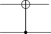
Basis Transformations and Reduction of Any Unitary Matrices . Unlike ideal classical gates, ideal quantum gates do not have high-impedance inputs. In fact, the role of “control” and “target” are arbitrary – they depend on what basis you think of a device as operating in. We have given the truth table for a CNOT and shown the control qubit does not get changed in the classical 00, 01, 10, 11 basis. However, in reality, the control qubit does change : its phase flipped depending on the state of the “target” qubit. One of example is demonstrated in Fig. 14.
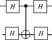
Figure 14. Basis Transformation of Hadamard gates and CNOT.
In order to realize arbitrary unitary transformations, single bit rotations need to be included. It was shown that CNOT with all one-bit quantum gates is a universal gate set. It suffices to include the following single bit rotations and phase shift transformations
Г cos a
sin a 1
V- sin a
cos a )
,
f ~ ia e
I 0
•)
e )
,
( ia
e
I 0
a 1 e )
.
We consider in this section the method that can to reduce any unitary matrix into a product of qubit rotations and CNOT`s. A qubit rotation acts on a single qubit at a time. We will discuss gates as CNOT`s that are state permutations that act on two bits at a time. Consider first the case when there are only two bits. Then there are four possible states: 00, 01, 10, 11. With these four states, one can build six distinct transpositions:
( 00,01 ) = f T x -L-1 = P ® a . + P 1 ® 1 2 = a . ( 0 ) n ( 1 ) (1)
-
V 11 2 )
( 00,10 ) = -! 2 0 = 1 2 ® P + T , ® P 0 = T x ( 1 ) n ( 0 ) (2)
-
V P 0 I P 1 )
I 2
,
( 00,10 ) =
( 00,01 ) =
P
V P 1 11 :
V
( 01,10 ) =
P-
P 0 )
: Tx )
V 1 r 1
x
V
= 1 2 ® P 0
= P 0 ® 1 2
)
,
+ T x ® P 1 = T x ( 1 ) n ( 0 )
+ P 1 ® T x = T x ( 0 ) ” ( 1 ) ,
where matrix entries left blank should be interpreted as zero. The rows and columns of the above matrices are labelled by binary numbers in increasing dictionary order. Note that the four transpositions (Positions (1), (2), (5), and (6)) change only one bit value. The other two transpositions (Positions (3) and (4)) change both bit value.
We will call (00, 11) the Twin - to - Twiner and (01, 10) the Exchanger . Expressions such as o, ( в ) n (“ ) where а Ф в are a special case of M x ( в ) M 2 ( в 2 ) , which was defined above. In this case o x ( в ) n ( “ ) equals ox ( в ) when it acts on a state for which n ( а ) = 1 , whereas it equals 1 if n ( а ) = 0 ; а is called the control bit and в the flipper bit .
Remark. The Exchanger has four possible representations as a product of CNOT :
|
1 |
( 01,10 ) = ( 01,00 )( 00,10 )( 01,00 ) = o x ( 0 ) n ( 1 ) o x ( 1 ) n ( 0 ) o x ( 0 ) n1 |
|
2 |
( 01,10 ) = ( 01,11 )( 11,01 )( 01,11 ) = o x ( 0 ) n "1 o x ( 1 ) n ( 0 1 o x ( 0 ) • ( 1 ) |
|
3 |
( 01,10 ) = ( 10,00 )( 00,01 )( 10,00 ) = ox ( 1 ) n ( 0 ) ox Wo ( 1 ) n ( 0 ) |
|
4 |
( 01,10 ) = ( 01,11X11,10X01,11 ) = o x ( 1 ) * o , ( 0 ) * ( 1 ) o x ( 1 ) "m |
We will often represent Exchanger by E ( 0,1 ) . It is easy to show that
|
1 |
ET ( 0,1 ) = E ( 0,1 ) = E -1 ( 0,1 ) |
|
2 |
E ( 0,1 ) = E ( 1,0 ) |
|
3 |
E 2 ( 0,1 ) = 1 |
Furthermore, if X and Y are two arbitrary 2 x 2 matrices, then, by using the matrix representation of Exchanger , one can show that E ( 0,1 ) ° ( X ® Y ) = Y ® X . Thus, Exchanger exchanges the position of matrices X and Y in the tensor product.
Twin – to – Twiner operator also has four possible representations as a product of CNOT . One is ( 00,11 ) = ( 00,01 )( 01,11 )( 00,01 ) = ox ( 0 ) n ( 1 ) ox ( 1 ) n ( 0 ) ox ( 0 ) n ( 1 ) . As with Exchanger , the other three representations are obtained by exchanging: (1) n and n ; (2) bit positions 0 and 1; (3) both.
Toffoli Gate. Tom Toffoli (1980) inspired by Bennet reversibility, investigate how reversible computing could be done in the traditional language of Boolean logic gates. He showed that a set of modified gates could be used in place of the traditional Boolean logic gates like AND, OR, etc. One of these, which has turned out to be of central importance in the subsequent quantum gate work is the CNOT gate and was discussed above. The simple retention of the source bit makes the CNOT gate reversible – the input is a unique function of the output. The target bit is transformed to the exclusive – NOT (XOR), while the source bit is unchanged. The CNOT gate is not universal for Boolean computation. Toffoli sought another reversible gate, which could play the role of a universal gate.
Remark. A “universal ” logic gate is one from which one can assemble a circuit which will evaluate any arbitrary Boolean function. In ordinary (irreversible) Boolean logic, NAND (or AND supplemented by NOT) is one choice for the universal gate.
The Toffoli gate ( double CNOT) requires three bits, symbolized in Fig. 15.
|
a |
|
|
a b |
|
|
b Л |
|
|
c c u |
c ⊕ (a ∧ b) |
Figure 15. The three – bit Toffoli gate is universal for reversible Boolean logic. The action of the gate on the three input bits is indicated
Any universal reversible Boolean logic gate must have at least three bits. In essence, this gate is an AND gate in which both input bits are saved; as Fig. 15 indicates, bits a and b are unchanged, while bit c is “toggled” by a ∧ b . The Toffoli gate is reversible classical gate which is universal for classical computation. The XOR is also a classical gate, but the only classical functions that can be constructed with it are linear Boolean functions; it takes three bits to provide a reversible classical gate, which is universal for classical computation (recall that all quantum gates must be reversible).
We will show to do both π / 2 rotations and Toffoli ( T ) gates fault – tolerant. The three – bit controlled – controlled –NOT (Toffoli) gate is also an instance of this conditional definition:
T = I 0>10 ⊗ I ⊗ I + I 11 I ⊗ CNOT .
T can be used to construct complete set of Boolean connectives in that it can be used to construct the NOT and AND operators in the following way:
|
T |
1,1, x = |
1,1, x |
|
|
T |
x , y ,0 = |
x , y , x ∧ y |
|
The quantum Toffoli gate is a three – qubit gate, as follows:
|
000 |
→ |
000 |
||
|
001 |
→ |
001 |
||
|
010 |
→ |
010 |
||
|
011 |
→ |
011 |
||
|
100 |
→ |
100 |
||
|
101 |
→ |
101 |
||
|
110 |
→ |
111 |
||
|
111 |
→ |
110 |
The T gate is sufficient to construct arbitrary combinatorial circuits.
Example . Consider the trivial example of a double controlled – NOT (Toffoli) gate, T , that computes the conjunction of two values as in Fig. 16.
|
x |
|
|
y |
|
|
0 |
I x
I y
I x ∧ y
Figure 16. Calculation scheme of the conjunction of two values with Toffoli gate
Now take as input a superposition of all possible bit combinations of x and y together with the necessary 0:
|
H 0) 0 H 0) 0 0) = |
^ ( 0 +11 )® ^ ( 0 +1 ) ®l 0) 1 ( 000) + 010) + 100) + 110) ) |
Superposition of inputs leads to superposition of results, namely
T ( H 0s) 0 H\ 0) 01 0) ) = 1 ( 000) +1 010) +1 100) +1 111) )
The resulting superposition can be viewed as a truth table for the conjunction, or more generally as the graph of a function. In the output the values of x , y , and x л y are entangled in such a way that measuring the result will give one line of the truth table, or more generally one point of the function graph. Note that the bits can be measured in any order: measuring the result will project the state to a superposition of the set of all input values for which the function f produces this result; measuring the input will project the result to the corresponding function value.
Example . Consider the application of T gate in quantum computation. Suppose we want to build a dedicated quantum device to factor large integers. The quantum factorization contains two major operations: quantum exponentiation (computing a x mod N ) followed by the Quantum Fourier transform. Quantum exponentiation can be decomposed into a sequence of squaring, ax = a 2 x 0 • a 2 x 1 •...• a 2 x l 1 , where x 0, X j,.. are the binary digits of x . Squaring is achieved by multiplication and multiplication by a sequence of additions. Following this reduction procedure we end up with a quantum adder as a basic unit for the whole network. However, a quantum adder is different from a classical adder. Any unitary operation is reversible which is why quantum network for basic arithmetic cannot be directly deduced from their classical Boolean counterparts (classical logic gates such as AND or OR are clearly irreversible – reading 1 at the output of the OR gate does not provide enough information to determine the input which could be either (0,1) or (1,0) or (1,1) ). Quantum arithmetic must be build ab initio from the reversible logical components.
A simplified quantum adder shown in Fig. 17.
Quantum adder
| xy Ф z
Toffoli
sum = | x e y)
CARRY =| xy)
Figure 17. Diagrammatic representation of the Toffoli gate and a simplified quantum adder. States x , y and | z) belong to the computational basis x , y , z = 0 or 1 and both addition e and multiplication x • y are performed modulo 2
The Toffoli gate is a basic unit which features prominently in the network implementing elementary quantum arithmetic, i.e. in quantum adders, multipliers etc. It can be decomposed and written as a quantum network of elementary two – qubit and one – qubit gates. The following quantum circuit, for example, implements a 1 bit full adder using T and CNOT gates (Fig. 18):
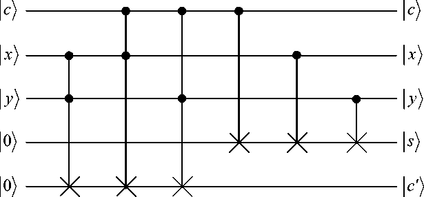
Figure 18. An one – bit full adder using Toffoli and CNOT gates
Where x and y are the data bits, s is their sum (modulo 2), c is the incoming carry bit, and c ' is the new carry bit. It is possible define more complex circuits that include in – place addition and modular addition.
A simplified quantum adder is a starting point for constructing more elaborate networks.
Example. How do we construct the Toffoli gate? One major problem with this gate is that it requires three bits in and three out. Quantum mechanically, this seems to correspond to a scattering process involving three – particle collisions calling for a (possible) unreasonable control of the particles. Fortunately, the Toffoli gate may be constructed by two – particle scattering processes. In particular, we show a construction here involving the CNOT gate and some one – bit gates U (Fig. 19).
B ©( A.C))
Figure 19. The Toffoli gate built from two – bit CNOT gates plus some one – bit gates. This circuit introduced some extra signs in the unitary matrix U which may be removed at a later stage
Not only is the CNOT sufficient for all logic operations in quantum computation, but it can be used to construct arbitrary unitary transformations on any finite set of bits.
The Fredkin Gate (F). The F gate is a “ controlled SWAP ” and can be defined as
F = |0>(0| ® I ® I + HOI ® S where S is the SWAP operation: S = 100^001 +10^101 +110^011 +111X111. The Fredkin (F) gate has the truth table as in Fig. 20.
|
Inputs |
Outputs |
||||
|
A |
B |
C |
A' |
B' |
C' |
|
0 |
0 |
0 |
0 |
0 |
0 |
|
0 |
0 |
1 |
0 |
0 |
1 |
|
0 |
1 |
0 |
0 |
1 |
0 |
|
0 |
1 |
1 |
1 |
0 |
1 |
|
1 |
0 |
0 |
1 |
0 |
0 |
|
1 |
0 |
1 |
0 |
1 |
1 |
|
1 |
1 |
0 |
1 |
1 |
0 |
|
1 |
1 |
1 |
1 |
1 |
1 |
B >
C >
A >
A ’
Figure 20. The truth table of Fredkin gate
The following table shows that F , like T , is complete for combinatorial circuits:
|
F |
x ,0,1) = |
x , x , — x) |
||
|
F |
x , y ,1 |
= |
x , y V x , y v ■ x) |
|
|
F |
x ,0, y |
= |
x , y л x , y л — x) |
|
The CNOT gate can be constructed from two Fredkin gates.
While the T and F gates are complete for combinatorial circuits, their cannot achieve arbitrary quantum state transformations. In order to realize arbitrary transformations, single bit rotations need to be included.
Decomposition of controlled - U , V Gates and Universality for Quantum Gates. As claimed above, the CNOT gate, when supplemented by a repertoire of one – bit quantum gates, is sufficient to perform any arbitrary quantum computation. Many important quantum computations are formulated quite naturally using this repertoire. This repertoire (CNOT plus one – bit gates) is “universal” for quantum computation in the sense that the Toffoli gate above is universal for reversible Boolean computation. We were able to make use of another important early discovery of Deutsch (1989), which was that three – qubit gates U are universal
|
for quantum gate constructions, where U |
has the “double |
- controlled” form |
|
( 1 |
0000 |
0 0 0 ^ |
|
0 |
1000 |
0 0 0 |
|
0 |
0100 |
0 0 0 |
|
0 |
0010 |
0 0 0 |
|
UD = 0 |
0001 |
0 0 0 |
|
0 |
0000 |
1 0 0 |
|
0 |
0000 |
0 u n u !2 |
|
v 0 |
0000 |
0 u 21 u 22 ? |
Here the uy constitute a generic U ( 2 ) matrix. This gate is a quantum generalization of the Toffoli gate. It is fortunate for the prospects for physical implementation of quantum computation that, unlike in Boolean reversible computation, the Deutsch gate can indeed be broken down into simple parts. The simplest means of achieving this decomposition is shown in Fig. 21.
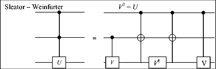
Figure 21. The construction showing the Deutsch three – qubit gate can be broken down into a series of two – qubit operations.
0 10о
V0 0 V,.
V 0 0 V 21 V 22 У
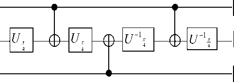
Here V is a U ( 2 ) matrix such that V 2 = U . These two -bit controlled - V gates could be further broken down, as shown in Fig. 22.
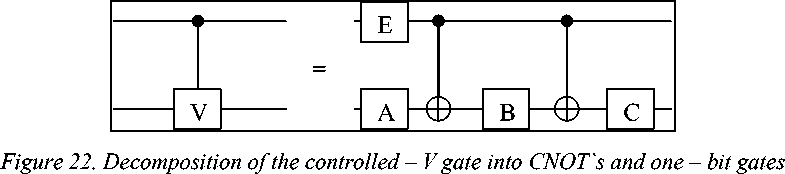
Here A, B, C, and E are one – bit gates for which can be obtained explicit formulae (see abovementioned description).
Thus, the circuits, elements which would be needed in any quantum computation in which we are currently interested can be readily be simulated by short sequences of two – bit gates. For instance, the Toffoli gate, which would be the basis of much of the ordinary Boolean logic which is needed for large sections of, for example, Shor prime factoring, can be obtained with just six CNOT`s and eight one – bit gates by using the constructions above (this is shown in Fig. 23).
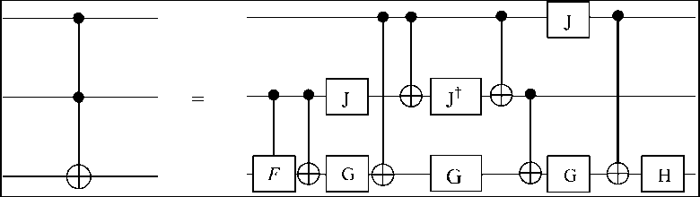
Figure 23. Simplest decomposition of the Toffoli gate into six CNOT gates and eight one – bit gates (operations F, G, H, and J in text are described)
The unitary operators for one – bit gates in this construction are eiin/4
F =
cos — n
e i n /4
—
eli I /4
Sin — П
e i n /4
H =
—П — i n / 4
0 )
■ 1 к
Sin-л cos -л
8 J
G =
cos — n
sin -л к__8_
. ( 1
■ 1 к
— sin - n 8
cos -n
8 J
к
i n /4
e J
J =
0 )
к 0 e
— i n /4
J
It may be noted that in this construction the gates can be grouped into a sequence of just five two – bit operations: first a 2 – 3 operation, then 1 –3, 1 – 2, 2 – 3 and finally 1 – 3 (numbering the qubits 1 – 2 – 3 from the top). Simulations have indicated that the Toffoli gate can be obtained with no fewer than five two – bit quantum gates of any type.
In a related result, Margolus has found an “almost” Toffoli gate which requires even less resources, as shown in Fig. 24: just three CNOT`s and four one – bit gates (three two – bit gates over).
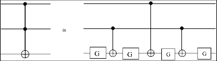
Figure 24. Margolus`s simplified Toffoli gate construction, if just one of the quantum phases is allowed to be changed
It is “almost” in the sense that one of the matrix elements of the Tofffoli gate is changed from 1 to – 1 (the one corresponding to the 100 state). This is not generally acceptable for quantum computation, where all the phases must be correct. However, in many quantum programmes the Toffoli gates appear in pairs, so that the “wrong” phase of the Margolus construction can be arrange to cancel out.
References Examples of quantum computing toolkit: Kronecker product and quantum Fourier transformations in quantum algorithms
- Gruska J. Quantum computing. - Advanced Topics in Computer Science Series, McGraw-Hill Companies, London. - 1999.
- Nielsen M.A. and Chuang I.L. Quantum computation and quantum information. - Cambridge University Press, Cambridge, Englandю - 2000.
- Hirvensalo M. Quantum computing. - Natural Computing Series, Springer-Verlag, Berlinю - 2001.
- Hardy Y. and Steeb W.-H. Classical and quantum computing with C and Java Simulations. - Birkhauser Verlag, Basel. - 2001.
- Hirota O. The foundation of quantum information science: Approach to quantum computer (in Japanese). - Japan. - 2002.
