Examples of quantum computing toolkit: Kronecker product and quantum Fourier transformations in quantum algorithms

Author: Reshetnikov Andrey, Tyatyushkina Olga, Ulyanov Sergey, Tanaka Takayuki, Yamafuji Kazuo
Journal: Сетевое научное издание «Системный анализ в науке и образовании» @journal-sanse
Article in issue: 3, 2017.
Free access
Quantum mechanics requires the operations of quantum computing to be unitary, and makes it important to have general techniques for developing fast quantum algorithms for computing unitary transformations. A quantum routine for computing a generalized Kronecker product is given. Applications for computing the Walsh-Hadamard and quantum Fourier transform is include also re-development of the according network.
Quantum computing, generalized kronecker product, quantum fourier transform
Short address: https://sciup.org/14123276
IDR: 14123276
Примеры инструментария квантовых вычислений: произведение Кронекера и квантовое преобразование Фурье в квантовых алгоритмах
Квантовая механика требует, чтобы операции квантовых вычислений были унитарными, и делает важным иметь общие методы для разработки быстрых квантовых алгоритмов вычисления унитарных преобразований. В работе представлена квантовая подпрограмма для вычисления обобщённого произведения Кронекера. Приложения для вычисления Уолша-Адамара и квантового преобразования Фурье включают в себя также проектирование соответствующей сети.
Text of the scientific article Examples of quantum computing toolkit: Kronecker product and quantum Fourier transformations in quantum algorithms
The fundamental object is the unitary transform, which then can be considered a quantum or a classical (reversible) algorithm. With point of view, the problem of finding an efficient algorithm implementing a given unitary transform U into small number of “sparse” unitary transforms such that those sparse transforms should be known to be efficiently implementable. As an example of this, the quantum networks implementing the quantum versions of the discrete Fourier transforms can be easily derived from the mathematical descriptions of their classical counterparts [1-18].
Remark . For simplicity, we will use Kronecker product. The other two names: direct product and tensor product are also similar [19, 20].
Remark . More generally, unitary transform can be expressed as a certain generalized Kronecker product (defined below) then, given efficient quantum network implementing each factor in this expression, we also have an efficient quantum network implementing U . The expressive power of the generalized Kronecker product includes several new transforms.
Generalized Kronecker products
All matrices through this Section are finite. Recall that a square matrix is unitary if it is invertible and its inverse is the complex conjugate of its transpose. The complex conjugate of a number c is denoted by c .
Let us introduce any definitions.
Definition 1 . Let c be a ( p x q ) matrix and C a ( k x l ) matrix. The left and right Kronecker product of
( p x q ) and C are ( pk x ql ) matrices
Definition 2 . Given two tuples of matrices, a k - tuple A = ( A ) of ( p x q ) matrices and q - tuple C = ( C ) q of ( k x l ) matrices, the generalized right Kronecker product is the ( pk x ql ) matrix D = A ®R C where
R vx ij uk+v, xl+y ux vy with 0 < u < p, 0 < v < k, 0 < x < q, and 0 < y < l.
Definition 3. The generalized left Kroneker product is the (pk x ql) matrix D = A ®L C where (г, j ) — th entry holds the value d.. = d = a" C ij up+v, xq+y vy ux with 0 < u < k, 0 < v < p, 0 < x < l, and 0 < y < q.
Remark . The left Kronecker product denoted by A ®^ C and the right Kronecker product denoted by A ®R C. when some property holds for both definitions, we use A ® C. The Kronecker product is a binary matrix operator as opposed to the tensor product which is binary operator defined for algebraic structures like modules. The Kronecker product can be generalized in different ways. We use the generalized Kronecker product defined in Definition 1 .
Remark . The generalized right Kronecker product can be found from the standard right Kronecker product by, for each sub-matrix a C in Definition 1 substituting it with the following sub-matrix
|
a ux C 00 |
a u 0 x c 0 x 1 |
• • aux C 0, l —1 |
) |
|
a u 1 x c 1 x 0 |
a u 1 x c 1 x 1 |
a o C 01 —1 |
|
|
ak — 1 cx V a ux c k —1,0 |
a "x1 c ix —1,1 • |
a k "xc x • • aux c k —1, l —] |
J |
Remark . As for standard Kronecker products, we let A ® C denote either of the two definitions. If the matrices A = A are all identical, and also C = C , the generalized Kronecker product A ® C reduced to the standard Kronecker product A ® C . Denote A ® C the generalized Kronecker product of a k — tuple A of ( p x q ) matrices, and q — tuple C of ( k x l ) identical matrices C . Denote A ® C similarly.
Example . Let us consider the differences between left and right Kronecker products.
|
Ar ^ u |
= |
< V |
"1 1 ■ .-1 - 1 - |
[ 1 0" , - 0 1 -. |
) ® R ) |
[ 1 1 - - 1 - 1 _ |
^ |
|||
|
[0 ■ 1 ) ( 11 ) ( 1 ■ 1 ) ( 1 ■ c - 1 ) ) |
( 11 ) (r 1 ) " ( 0 1 ) ( 0 ( - 1 ) ) |
= |
1111 - 1 - 1 0 0 1 1 - 1 - 1 0 0 1 - 1 - |
|||||||
|
( 1 ■ 1 ) (M) ^ ( 04) ( 0 ■ ( - 1 ) ) |
(Hh0 (( - 1 )■O ( 11 ) ( 1 ( - 1 ) ) |
|||||||||
|
Al ^ u |
= |
( V |
■ [ 1 1 ■ .- 1 - 1 - |
[ 1 0 ., - 0 1 - |
^® L / |
[ 1 1 - - 1 - 1 _ |
^ |
|||
|
[ ( 11 ) ( 11 ) ( b1 ) ( ( - 1 ) ^) |
(ы) ( 11 ) ~ (i 1 ) ( ( - 1 ) ^) |
= |
1111 - 1 - 11 - 1 1 0 - 1 0 0 10 1 _ |
|||||||
|
( b1 ) (0^) ^ (0d) ( b1 ) |
( 1 ( - 1 ) ) ( 0 ( - 1 ) ) ( 0 ^ ( - 1 ) ) (r( - 1 ) ) . |
|||||||||
Thus, as result AR * AL , i.e., left and right Kronecker products are non-commutative relation.
To analyze generalized Kronecker products we need the shuffle permutation matrix of dimension (mn x mn ) , denoted П (as shorthand for П A, defined by
\ / , mn v ( m,n ) ',
^rs = ndn+I,d'm+I' = ^dl'^d1 , where 0 < d, I' < m; 0 < d', I < n, and d. denotes the Kronecker delta function which is zero if x * y, xy and one otherwise. It is unitary and satisfies П-^ = ПTmn = Птn. Given two tuples of matrices, k-tuple A = ( A ) of (p x r) matrices and k - tuple C = ( C )q of (r x q) matrices, let A ■ C denotes the k - tuple where the i-th entry is the (p x q) matrix A1 C , 0 < i < k . For any k - tuple A of matrices, let k-i _ diag (A) denote the direct sum Ф Ai of matrices A0,.., Ak-1. The generalized Kronecker products satisfy the following important diagonalization theorem.
Theorem ( Diagonalization theorem ): Let A = ( A1 ) be a k - tuple ( p x q ) matrices and C = ( C ) q a q - tuple of ( k x 1 ) matrices. Then
|
A ®„ C R |
= |
( П pk diag ( A ) П kq ) x |
diag ( C ) |
||
|
A ®£ C |
= |
diag ( A ) |
x ( n ,, d/ag ( C ) П q ) |
||
.
Corollarl : Let A = ( A i ) be a k - tuple ( p x q ) matrices and C = ( C ) q a q - tuple of ( k x 1 ) matrices. Then
|
A ®R C R u |
= |
П pk |
( A ® L C ) |
П q |
|
u |
||||
|
A ®L C |
= |
П kp |
( A ® . C ) |
П q1 |
Remark . Until now, we have not assumed anything about the dimension of the involved matrices. In the text theorem, we assume that the matrices involved are square matrices. The theorem is easily proven from
Diagonalization theorem . For any k — tuple A =
( A
k-1
) i =0
of invertible matrices, let A-1 denote the k — tuple
where i -th entry equals the inverse of A , 0 < i < k .
Corollary : Let A, C be m -tuples of ( n x n ) matrices, and D, E be n -tuples of ( m x m ) matrices.
Then
AC a DE
(AaIm)x(CaD)x(In aE)
Furthermore, if the matrices in the tuples A and C are invertible, then
|
f )—1 A ®„ C R к я J |
= |
n..... ( C -1 a , a -1 ) n..... |
= |
C - 1 a L A -1 я |
|
( a a l c )" |
= |
П ( C-1 a L a ) n |
= |
C-1 a R A-1 |
If A and C are unitary then so is A ® C .
Quantum routines (A method for constructing a quantum network for computing any given generalized Kronecker product.) A primary application of this method is a tool to find a quantum network of a given unitary matrix.
As our quantum computing model, we adopt the now widely used quantum gate arrays. Let т : \u , v^ > | u , v Ф u^ denote the two-bit exclusive-OR operation, and U the set of all one-bit unitary operations. By a basic operation we mean either a U operation or the т operation. The collection of basic operations is universal for quantum networks in the sense that any finite quantum network can be approximated with arbitrary precision by a quantum network Q consisting only of gates such operations. Define the one-bit unitary operations
|
X |
= |
Г 0 1 ) к 1 0 J |
Z |
= |
Г 1 0 ) к 0 —1> |
Y |
= |
Г 0 — 1 ) к 1 0 v |
H |
= |
1 Г 1 1 ) N 2 к 1 1 J |
Given a unitary matrix C. let Л ( ( j , x ) , ( k , £)) denote the transform where we apply C on the k -th register iff the j -th register equals x . Given an n -tuple C— { C i} _ of unitary matrices, let Л ( ( j , i ) , ( k , C )) denote л ( ( j , n — 1 ) , ( k , C n — 1 ) ) • • *Л ( ( j , 0 ) , ( k , C 0) ) . Given a k -th root of unity, say to , let Ф ( to ) denote the unitary transform given by | u}|v ) > touv |u}|v ) . If the first register holds a value from Xn , and the second holds a value from Zm, then Ф ( to ) = Ф^т) ( to ) can be implemented in ® (Г log nA Г log mA ) basic operations.
Example : Typical matrix operations . Let us consider the implementation of the following operations.
-
1 . Quantum shuffle transform
-
2 . Quantum direct sum
-
3 . Quantum Kronecker product
Let the operation DMm perform the unitary transform k |0) > |kd/vm^|k mod m^ , for every m > 1. Let SWAP denote the unitary transform |u)|v) —SWAP > | v)|u) . Then Птп can be implemented on a quantum computer by one application of DMm , one SWAP operation, and one application of DMm 1, i.e., П = DM-1 SWAPDM. mn m m
Let C be an n -tuple of ( m x m ) unitary matrices. It is true that Diag (C) can be implemented as follows,
Diag (C) = DM - Л ( ( 1, i ) , ( 2, C i )) DM m .
In general, the time to compute the direct sum is proportional to the sum of the computation times of each of the conditional C i transforms. However, if parts of these can be applied in quantum parallel, this improves the running time.
Let A be an m -tuple of ( n x n ) unitary matrices and C be an n -tuple of ( m x m ) unitary matrices. By the Diagonalization theorem, the generalized Kronecker product can be applied by applying two direct sums and two shuffle transforms. Removing canceling terms we get
A ® R C = DM-> ( ( 2, i ) , ( 1, л # )) л ( ( 1, i ) , ( 2, C i )) DM m
A ® L C = DM - л ( ( 1, i ) , ( 2, A )) л ( ( 2, i ) , ( 1, C i )) DM n .
Thus, an applications of a generalized right Kronecker product can be divided up into the following four steps: in the first step, we apply DM . In the second step, we apply the controlled C i transform on the second register, and in the third step, the controlled A i transforms on the first register. Finally, in the last step, we apply DMw 1 to the result.
Example . Let A be a 4-tuple of ( 2 x 2 ) unitary matrices, and C a 2-tuple of ( 4 x 4 ) unitary matrices. The generalized Kronecker product A ®R C can be implemented by a quantum network. The dots and the circles represents control-bit: if the values with the dots are one, and if the values with the circles are zero, the transform is applied, otherwise it is the identity map. The least (most) significant bit is denoted by LSB (MSB). Note that the most of the transforms are orthogonal, and thus the gates commute.
Remark . Following the ideas of Griffiths et all , a semi-classical generalized Kronecker product transform can be defined.
Properties of the Kronecker product in quantum information theory
We will discuss the properties and applications of Kronecker product in quantum theory that is studied thoroughly. The use of Kronecker product in quantum information theory to get the exact spin Hamiltonian and the proof of non-commutativity of matrices, when Kronecker product is used between them is also given. The non-commutativity matrices after Kronecker product are similar or they are similar matrices.
Remark . The use of Kronecker product in quantum information theory is used extensively. But the rules, properties and applications of Kronecker product are not discussed in any quantum textbooks. Even books on mathematical aspects of quantum theory are discussed the properties and applications of Kronecker product in very short without any explanations of its rules. That is, why we applying Kronecker product left/right to any spin operator, why not left or why not right only. They are applying Kronecker product without any explanation. Mathematicians were also not able to give any concrete answer to these questions in more generalized way. We can find textbooks on algebra, where the mathematical aspects are considered in more rigorous and detail. But many books on algebra do not consider the physical aspects of Kronecker product, which are very important in quantum theory. So, we will discuss answers to all of the abovementioned questions, which are now very important in quantum information theory to write exact spin Hamiltonian.
Mathematical aspects of Kronecker product
Let A and B are two linear operators defined in the finite dimensional L and M vector spaces on field
-
F . A 0 B is the Kronecker product of two operators in the space L 0 M. Kronecker product of two matrices
are given by the rule: ( A ) , , 0 ( B ) „ „ = ( C ). , _, ,
After the Kronecker product the dimensions of
b A ) ml, n 1 X /m 2, n 2 V /( m 1, m 2 ) , ( n1, n 2 )
the finite space becomes N • M , where N and M are dimensions of finite spaces on which operators A and B are defined.
Properties of the Kronecker products. Let the operators A ˆ1, A ˆ2, B ˆ1, B ˆ2 and E ˆ (unity matrix) are defined in finite dimensional vector spaces L1, L2, M1, M2 and E ˆ is defined in L1, L2, M1, M2 on the field F . The properties of the Kronecker product can be written as following (see Table 1).
Table 1. The properties of the Kronecker product
|
N |
Kronecker product property |
|
1 |
( A 1) , , 0 0 = 0 0 ( B 1) , = 0 ( 0 is zero matrix ) m 1 n 1 m 1 n 1 |
|
2 |
( E ) , , 0( E ) , , =( E ) , ,w , x / m 1, n 1 X m2 2, n 2 x /( m 1, n 1 ) , ( m 2, n 2 ) |
|
3 |
{( A 1 ) , , +( A 2 ) , J0( B 1 ) , , =( A 1 ) , , 0( B 1 ) , , +( A 2 ) , , 0( B 1 ) , , m 1, n 1 m 2, n 2 m 1, n 1 m 1, n 1 m 1, n 1 m 2, n 2 m 1, n 1 |
|
4 |
( A 1 ) , , 0(( B 1 ) , , +( B 2 ) , J = ( A 1 ) , , 0( B 1 ) , , +( A 1 ) , , 0( B 2 ) „ „ m 1, n 1 m 1, n 1 m 2, n 2 m 1, n 1 m 1, n 1 m 1, n 1 m 2, n 2 |
|
5 |
s • ( A 1 ) , ,0 t • ( B 1 ) , = s • t • ( A 1 ) , , 0 ( B 1 ) , ,( s , t are constants ) m 1, n 1 m 1, n 1 m 1, n 1 m 1, n 1 |
|
6 |
(( A 1 ) , , 0 ( B 1 ) , Г* = ( B 1 )- 1 , 0 ( A 1 )- 1 , m 1, n 1 m 1, n 1 m 1, n 1 m 1, n 1 |
|
7 |
(( A 1) , ,•( B 1) , ,)0{( A 2) , •( B 2) , J = (( A 1) , , 0( A 2) , JV( B 1) , ,0( B 2) , J m 1, n 1 m 1, n 1 m 2, n 2 m 2, n 2 m 1, n 1 m 2, n 2 m 1, n 1 m 2, n 2 |
|
8 |
(( A1) , , 0 ( B 1) , ,)#(( B 1) , , 0 ( A 1) , ,) m 1, n 1 m 1, n 1 m 1, n 1 m 1, n 1 |
Example . We will prove only one property (8), which is used in quantum information theory. The others can be proved easily by analyzing the proof of property (8).
Theorem: The Kronecker product of two matrices are non-commutative, i.e.
( ( A 1 ) . ,, . 1 0 ( B 1 ) 2 ,1,1 ) * ( ( B 1 ) 21.1
0 ( A 1 ) „, . 1 ) .
Proof. Let two linear operators A ˆ and B ˆ with bases a and b are defined in finite vector spaces L and M vector spaces on field F . The operators can be written into the form of matrices ( A) and (B) . First we will write the L.H.S part of the Kronecker product, i.e., ( A ) 0 ( B ) and then R.H.S ( B ) 0 ( A ) . Then, we will compare all the elements of both the L.H.S and R.H.S matrices. If even one of the element with same indices of both the matrices differ then these matrices are not equal or non-commutative.
|
( A ) m x n |
0 ( B ) m x n |
= |
( A i( B ) 1,1 X /m x n A 2,1 ( B ) m x n |
A 1,2 ( B ) m x n A 2( B ) 2,2 x /m x n |
••• A Л B ) ) 1, n X /m x n A ,,( b ) 2, n X /m x n |
(5) |
|
|
. Am 1( B ) m ,1 m x n |
Am 2( B ) m ,2 m x n |
- a.. ( B ) m x n J |
|||||
|
( B ) X / m x n |
0 ( A ) x / m x n |
= |
B 1,1 ( A ) m x n B 2,1 ( A ) m x n • • • |
B 2( A ) 1,2 m x n B 2,2 ( A ) m x n |
1, n ( )m x n - B 2, n ( A ) . x n ... ... |
(6) |
|
|
I B -J ( A )...... |
Bm ( A A ) m ,2 m x n |
. , n ^^^m x n J |
The elements of both matrices are not equal. It means that these matrices are non-commutative.
Remark. Only the Kronecker product of two unity matrices are equal, i.e., they are commutative.
Similar operators (matrices)
ˆˆ
Let two linear operators A and B with bases a and b are defined in finite vector spaces L and M vector ˆ spaces on field F. The question arises, when operators A and B are considered similar. Since, we are interested in the similarity of these operators, so we will study the action of these operators on different bases in different vector spaces.
Definition: The operators A: L ^ L and B : M ^ M are called similar operators, if they are defined on field F, dim A = dim BB and exist isomorphism f : L ^ M , i.e., BB (b) = f A f 1 (b).
For this case we have the following theorem.
|
Theorem : If operators A ˆ and B ˆ with bases (a) and (b) are defined in vector spaces L and M on field F then the matrices of operators A ˆ and B ˆ in their corresponding bases a and b are similar, i.e., ( A ) a = ( B ) b . |
||||
|
Proof. Let the bases ci : av...,an and b : f ( L ^ M )( a ) = ax \.. ,,an ' of linear operators J l and BB are defined in vector spaces L and M on field F then |
||||
|
A ( С ) |
= |
Z A - „( a , ) i |
. |
|
|
BB ( b ) |
= |
B1 f ( a , ) = f A ( , ) |
||
|
= f Z A i ( a , ) i |
= |
Z Aj ( a , ) = Z A i ,( a ') |
||
|
Hence, A and are similar matrices |
||||
Example : More simplified proof of theorem . Let the linear operator C ˆ defined in vector space L and M changes the bases a into b , i.e.,
|
b j |
= |
Z C-.a , (7) i |
Aa |
= |
Z A -,, a , (8) i |
The operator A acts on basis b gives the matrix D and basis vector b
|
Bˆb j |
= |
Z B, , b - (9) i |
Aˆb j |
= |
Z D -, b - d°) i |
By putting (7) into L.H.S. of (10)
a ZC-A = ZCk..,A °k = ZZ' a(11)
k kki
By putting (7) into R.H.S. of (10)
ZDkjbk =ZDk,ZC.A = ZZC-A^i .(12)
k k iki
The R.H.S. of (11) and (12) are equal
C-A, = A,A, or
(D )=(C)" •( A )•(C).
The theorem is proved.
Physical aspects of Kronecker product and its applications in quantum information theory
The Kronecker product in group theory is widely used, especially with Wigner D-function. The main purpose of its use in physics is to get the higher dimensional vector space. For example, in atomic physics, when we want to calculate the eigenvalues and eigenvectors of a system of spins ½ or spin Hamiltonian.
We analytically or with help of PC diagonalize spin Hamiltonian and find eigenvectors and eigenvalues with two methods:
Remark . But there are some mathematical and physical problems during the process of Kronecker product. These problems are can be described as following.
|
( a ) |
As it seen from the non-commutative nature of Kronecker product that we do not have right to take Kronecker product for two different spins freely (because they are non-commutative). Then how Kronecker product can be applied in quantum theory. |
|
( b ) |
The non-commutative matrices [ ( A ) ® ( B ) ^ ( B ) ® ( A ) J after the Kronecker product are called similar matrices. It means, the eigenvalues of matrix ( AB ) = ( A ) ® ( B ) and ( BA ) = ( B ) ® ( A ) are similar. But eigenvectors of some eigenvalues are misplaced with their neighbourhood eigenvectors. This misplacement can be removed by applying the similar matrix method, which is proved earlier. The similar matrix method becomes more complicated as the dimensions of the vector space increases (number of spins increases). |
We will be discussed all of these problems below.
Applications in quantum theory
At the moment the Kronecker product is extensively used in quantum information theory. So, we concentrate on the applications of Kronecker product in information theory. All the applications of Kronecker product in quantum information theory can be easily applied to any other branch of quantum theory where it requires. Examples of Kronecker product are discussed below.
Example A2.1 : Hamiltonian of n spins ½ in Nuclear Magnetic Resonance (NMR) .
Let 0 t,..., 0n are linear spin operators defined in the finite dimensional ^ ,..., Sn vector spaces on field
F. g\ ® 02... ® 0n are defined in linear space St ® S2... ® Sn. All the matrices of spin operators д\v,0n are 2x2 dimensions. For simplicity, we are taking Й = 1.
-
1. Case n = 2 spins ½.
-
2. C ase n = 3 spins ½.
Hamiltonian of two spins 0x and 02 defined in linear space S1, S2. 0Xz and 02z coupling with hyper line interaction J12 are placed parallel to applied constant magnetic field Bo 11 - axis:
H2 = -HB0 ' (0z 1 ® E2 ) - M • (E1 ® 0z2 ) + J12 (°d ® 0,2 ) + J12 (0y 1 ® 0y2 ) + J 12 (0z 1 ® 0z2 ) •
Hamiltonian of three spins
H = -цВ0 ■ (< 7 Z, ® E2 ® E3 ) - ^b0 ■ ( Ex ® 7 2 ® e, ) - ^b0 ■ ( Ex ® / 1 ® 7 3) + J\2 (< 7 ,1 ® 7 2 ® E:3 ) + J 23( E :x ® c r2 ® < r 3) + j3 ,(< 7 -3 ® 7 ® E:2 ) Hamiltonians of higher spins ½ can be written in the same way as for 2 and 3 spins ½.
Kronecker product in quantum information theory to get the spin Hamiltonians
To write the spin Hamiltonian, first of all we should write S , S , S , S and then add them with their
corresponding factors, we will get the spin Hamiltonians (e.g., H and H ). We will proof this later.
Example . Let we want to write the spin Hamiltonian of n spins in NMR :
Total projection of n spins ½ on z-axis is conserved:
S ˆ
7,
n
® E i=2 i
if n = 1
+ Д ® CT2 z«
+ Ex ® E2 ® 73 z ^
n
® e , i=3 i
® Е5Х i =4 i
1 0
if n = 2
if n < 2
if n = 3
if n < 3
^ +...
The first term in Eq.(13) contains first spin < 7 lz with Kronecker product of E, unit matrices of other spins, i.e., second, third and so on. The second term contains first factor unit matrix E ˆ with Kronecker product of second spin < 72z and unit matrix of other spins. The third and forthcoming terms are
written analytically by analyzing preceding. Sx and S, can be written by putting 7 and 7 in place of 7 "z.
The square of the total spin S = S I S + 1 ) is conserved and
S ˆ
iS ,x + jS, + kS z ( 14 ) S
s x + s 2 + s 2 ( 15 )
Equations (14) and (15) are constant of motion. That is ^ Sz, S 2 J = 0 . It means that the eigenvalues and eigenvectors of (13) and (15) are identical.
The Hamiltonians H and H are consist of two parts (13) and (15) with their corresponding factors.
Example : Proof of H . To proof H , that it consists of (13) and (15), we should take two spins S and
/У /У
S 2 with constants at , i e x, y , z . To write Sx , Sy and Sz , we use (13), i.e.,
S; = a (<71 z ® E2 + eE,®,t2 z),
ˆ 2 ˆ 2 ˆ 2 ˆ 2
S 1 = S x + S y + S z
where
S’ = (<7,, ® Е1 )(Е ® 72, ) + (<7,, ® Е2 )(Е1 ® <72, )+ (<7,. ® Е2 )(<7,, ® Е2 ) + (<7,, ® Е2 )( Е ® 72, ) . (18)+ (Е ® <72x )(<71. ® Е2 ) + (Е ® 72x)(Е ® <72x)
By using the property (A2.8), we can simplified Eq. (18) to
S ˆ x 2
= 2ax [(Е, ® Е ) + (<7, x ® <72x)_ .
Similarly, we can calculate S ˆ 2 and S ˆ 2
S ˆ x 2
S ˆ z 2
= 2и; [(Е ® Е2 ) + (<7, у ® <72у)_, = 2а; [(Е1 ® Е ) + (<7, z ® <72z)'.
Now we will add (16), (19), (20), and (21) as following
S z + 5S 2 + S ? 2 + S 2 = a z (< 7 1 z ® Е2 + Е: 1 ® СУ 2 z ) + 7 x2 [ ( Е Т 1 ® Е2 ) + (,& xx ® С У 2 x )
+ 2 a y 2
( Д ® Е2 ) + ((Г1 у ® 72у )
+ 2U2 [(Е1 ® Е2 ) + ((71 z ® СУ2z )
By analyzing (22) and H , we can see that they are same, only we have to choose corresponding a .
The term 2 a 2 ( Е Г, ® Е Г2 )
does not have meaning, since it is unit matrix. We have proved that H can be correctly chosen with help of S
and S 2 using the properties
|
7 1 x ® < 7 2 x |
= |
<7 2 x ® < 7 1 x |
|
(71 у ® <7 2 у |
= |
<7 2 у ® <7 1 у |
|
^ z ® <7 2 z |
= |
<7 2 z ® <7 1 z |
The proof of H can be written similarly by applying property (8).
Similar matrices in quantum computation
Tensor product, which is very widely, used in quantum theory plays an important role not only for obtaining the higher dimensional Hilbert space but also to optimize the experimental technique. Since, the tensor product is non-commutative in nature, i.e., it cannot be applied freely to any operator without any knowledge of the constituents of the physical system. One very important property of tensor product is similar matrices, which have two optimization properties: reduces the number of pulses to realize some operator in physical experiment; and provides different choices of pulse propagations along different directions of axes. These two properties will be discussed with concrete physical realization of CNOT operator and how we can optimize its realization. We present theoretical result, which is based on the linear algebra (similar operators). The obtained theoretical results optimize the experimental technique to construct quantum computation e.g., reduces the number of steps to perform the logical CNOT (XOR) operation. The present theoretical technique can also be generalized to the other operators in quantum computing and information theory.
CNOT operator gates and CNOT’s similar matrices in quantum computing.
CNOT gates or similar matrices play an important role in the construction of quantum computation. All the complex quantum algorithms are based on the computation of NOT and CNOT logical gates or matrices in quantum computation. Here, we will not discuss the NOT logical gate or matrix, which is very simple negation operation. We will go in deep the mathematical and physical nature of CNOT logical gates. The other complex gates can be constructed on the basis of CNOT logical gates. Moreover, the construction of CNOT matrices plays an important role in quantum computation. Here, we will show that CNOT-matrices can be optimized by using the similar matrices, i.e., we can find different CNOT matrices with the same mathematical properties but some different experimental or physical realization. For better insight to understand the physical nature of similar matrices, we will discuss in the whole item the system of two spins ax = ^ and a2 = -^ with slightly different resonance frequencies o and o2, and having scalar coupling o12. The Hamiltonian of the two spins aligned along the z-axis with the constant magnetic field
H = OoxaXz ® e + Wo?ex ® a 2z + / о12а ь ® a2z , (23)
where c? , i g { 1, 2 } is identity matrix with 2 x 2 -dimensions .
Physical differences between the CNOT matrices.
Let us consider the CNOT matrix that contains additional spin a 1 rotation around the z-axis, which is unnecessary and which complicate the experimental realization of the CNOT as compare to the CNOT matrix used in NMR -quantum computation ( Gershenfeld and Cory , 1997 – 2002; Jones , 1998 - 2002). In the mathematical viewpoint, CNOT matrices have in this case different mathematical properties, i.e., CNOT matrices are not similar matrices due to the additional rotation of spin 6zX around z -axis.
Remark . Moreover, additional rotation takes more time to fulfill the CNOT operation, which slows
down the computation of quantum algorithms. The Gershenfeld is
CNOT matrix for Hamiltonian (23) obtained by
C g =

0 00
1 00
0 01
0 10
Physically, the C matrix was obtained by the following pulse sequences
C G
I П I П I ПI
= exp < - г — с? ® a. > exp < - г — a ® e > exp < - i — e ® a>
I 41 y2 I I 4 z1 2 I I 4 1 z2
1 П II x exp < г ~azX ® azl > exp < г — e ® az2
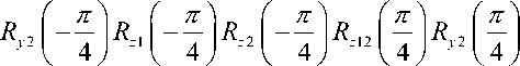
where R is rotation matrix around the different axes along with the different angles around different axes. The physical interpretation of the matrix R is just the rotation of our physical reference system or quantum tomography.
|
Remark . The two CNOT matrices for Hamiltonian (23) obtained by Cory are |
|||||||||
|
c C 1 |
= |
^ 1 0 0 0л 0100 0 0 0 1 v 0 0 - 1 0 ? |
c C 2 |
= |
л 1 0 0 0л 0 0 0 1 0 0 10 v 0 - 1 0 0 ? |
(26) |
|||
In the experiment of NMR , the CNOT matrices (26) are called Pound-Overhauser operators, i.e., transformation of spin polarization from one spin to other spin.
The C and C matrices were obtained with the following pulse sequences
|
C c 1 = Rx 2 | |
\ 1 EE \ 1 1 1 \ EE \ n п п п n R? R i? R i? R y? v 4 J z2 ( 4 J z 12 ( 4 J z 12 ( 4 J x 2 ( 4 J |
|
: : ТЕ : : • ~ z~x ^ i = exp j- i^e ® <7x 2 |
I П I I П I I • П ^/ГХ I > exp < - i — e. 0 a ~ exp < i — aA 0 a ~ > exp < i — e 0 a , > r1 4 1 z 2 1 ^1 4 z 1 z 2 1 ^1 4 1 z 2 1 |
|
C 2 | = | Rx 1 | |
теЛ ( te A ( te A ( те Л ( те Л п п П П п v 4 J z 1 ( 4 J z 12 ( 4 J z 12 ( 4 J x 1 1 4 J |
|
: : \ EE ( = exp j- i^ax i 0 e 2 |
I П I | П I 1 П I f exp j- i-<7z 1 0 e 2 [ exp j i ~az 1 0 az 2 Г exp j i ~ax 1 0 e 2 Г |
Mathematical differences between the CNOT matrices (24) and (26). Since, the Hamiltonian of the CNOT matrices (24) and (26) are the same but they are not similar matrices. To check the mathematical nature of (24) and (26), first of all we will write six mathematical properties of similar square matrices A and B of dimensions 4 x 4 on the Hilbert space H . _________________________________________________
|
1 |
Determinant of A is equal to determinant of B |
|
2 |
Trace of A is equal to trace of B |
|
3 |
If A and B are nonsingular than A 1 and B ' are also similar matrices |
|
4 |
A and B are similar matrices, if there exist nonsingular matrix P such that B = P4 AP or PBP4 = A |
|
5 |
Matrices A and B have the same eigenvalues |
|
6 |
PB_, = Aom, , where В_л, and Am, are the eigenvectors of the matrices A and B egv egv , egv egv |
The proof of above six properties of similar matrices is very simple and can be found in the course of linear algebra.
By applying six properties of similar matrices to the CNOT matrices (24) and (26), we will find that the properties second, fourth, fifth and six are not satisfied between CNOT matrices (24) and (26). Thus, the matrices (24) and (26) are not similar.
Physical interpretation of similar matrices
The similar matrices are very important part of the linear algebra in quantum computation. For example, by finding all similar matrices, we can get all the CNOT matrices or operators, which will reduce our mathematical and physical realization of quantum computing. If we apply all the six properties of similar matrices to CNOT matrices (26), we will see that matrices (26) are similar matrices. Now, if we apply operators C ci and C c2 to the state | ^ = a\ 0,0) + b | 0,1) + c | 1,0) + d |1,1) , of Hamiltonian (23). We will obtain
|
1 ^ 1) |
= |
C C 1 | v) |
= |
л 1 0 0 0 л 0 10 0 0 0 0 1 v 0 0 - 1 0 ? |
f a ( 0,0 ) ' b ( 0,1 ) c ( 1,0 ) V d ( 1,1 ) j |
= |
f a ( 0,0 ) ^ b ( 0,1 ) d ( 1,1 ) v- c ( 1,0 ) J |
|
|
1 v^ |
= |
C C 2 | v V |
= |
л 1 0 0 0 ^ 0 0 0 1 0 0 10 v 0 - 1 0 0 v |
f a ( 0,0 ) ' b ( 0,1 ) c ( 1,0 ) V d ( 1,1 ) j |
= |
f a ( 0,0 n d ( 1,1 ) c ( ,0 \ V- b ( 1,0 ) J |
the state ^ 2 у , which is obtained by operating C cl and Cc 2, and which gives us simple picture of the state before and after the CNOT operation. We can find all the CNOT matrices or similar matrices of (26).
Remark . Similar matrices of CNOT matrix (24) are have additional rotation, which complicates CNOT operation and which is not required for the CNOT operation. So, we are will find the similar matrices (26), which minimize CNOT operation in quantum computing.
CNOT similar matrices. As it is seen from the Eqs (27) that the state |0,0) in | ^ ) is not used by the CNOT matrix. It means, we have still more options to use the possibility to get other CNOT matrices or similar matrices. This can be done by considering the six similar matrix properties.
|
c C 11 |
= |
f 1 0 0 0 ^ 010 0 0 0 0 - i v 0 0 - i 0 v |
c C 51 |
= |
1000 0 0 0 - i 0010 0 - i 0 0 |
||||
|
c C 22 |
= |
л 1 0 0 0 ^ 0 0 0 - i 0010 v 0 - i 0 0 v |
c C 52 |
= |
' 1 0 0 0 л 0100 0 0 0 i v 0 0 i 0 v |
||||
|
c C 31 |
= |
f 0 0 - i 0 0100 - i 0 0 0 v 0 0 0 1 v |
c C 61 |
= |
' 1 0 0 0 ' 0 0 0 - 1 0010 , 0 10 0 , |
||||
|
c C 32 |
= |
л 0 - i 0 0 - i 0 0 0 0010 v 0 0 0 1 v |
c C 71 |
= |
' 0 - 1 0 0 " 1000 0010 v 0 0 0 1 v |
||||
|
c C 11 |
= |
л 1 0 0 0 ^ 010 0 0 0 0 - i v 0 0 - i 0 v |
c C 72 |
= |
' 0 0 - 1 0 " 01 00 1000 v 0 0 0 1 v |
||||
|
c C 41 |
= |
' 0 0 10 ^ 0 10 0 - 10 0 0 v 0 0 0 1 v |
c C 81 |
= |
' 0 i 0 0 ^ i 0 0 0 0 0 10 v 0 0 0 1 v |
||||
|
c C 42 |
= |
' 0 10 0 л - 1 0 0 0 0 0 10 v 0 0 0 1 v |
c C 82 |
= |
' 0 0 i 0л 0100 i 0 0 0 v 0 0 0 1 v |
We have obtained 16 CNOT matrices or operators, which are obtained by using the similar matrices properties. It means we can perform the CNOT operation on qubits with different pulse rotations around the different axes according to this convenience. The technique of similar matrices is very closely related to the tensor product, which was above described. The similar matrices method can be applied to the other branches of quantum theory.
The Quantum Fourier Transform and Algorithms Based on It: From DFT to QFT
The classical discrete Fourier transform (DFT) on N input values (28), is defined as
N -1
-
У , = -—£ - ,0 < k < N - 1 ,
V N j =0
with a)N : = e ^iN denoting the Ntk root of unity. Its inverse transformation is x. = —^ £ N o1
y k ^ N .
Remark. In some quotations the coefficient is 1 N instead of 1 N . In this case, the inverse transformation has no factor 1 N . If the x are values of a function f at some sampling points, it is often written f instead of x and f ˆ instead of y .
Considering the different notations the quantum Fourier transform (QFT) corresponds exactly to the classical DFT in (28). Here, the QFT is defined to be the linear operator with the following action on an
N -1 N -1
arbitrary n-qubit state: £ ^ I. QFTL £ >М j=0 k=0
Remark. In literature the definition of the Fourier transform is not consistent. The DFT and its inverse transform are interchanged. In most original papers the QFT is defined as above. However, both the classical Fourier transform and its inverse transform can be deduced from the general form of a Fourier transform with N = 2 n . The yk are the Fourier transforms of the amplitudes x. as defined in Eq. (28). In product representation, the QFT looks like
,2ni 0. jn
>
11 )(| 0) + e ^ni 0. j n - 1 j n
2 n 2
+ e 2 n i0- j1 j 2 - j n
.
This leads to an efficient circuit for the QFT which is shown in Fig. 1.
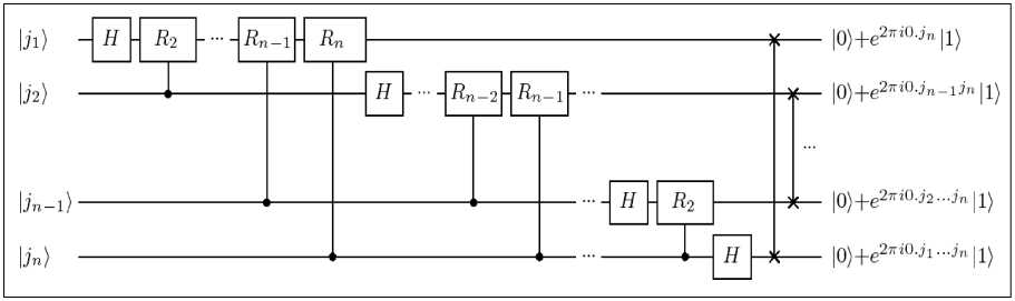
Figure 1. A Quantum circuit for QFT
The gate Rk corresponds to the phase gate PH (2nj2k ). At the end of the circuit, swap gates reverse the order of the qubits to obtain the desired output. The circuit uses n (n -1)/2 Hadamard and conditional phase gates and at most n 2 swap gates in addition. Therefore, this n-qubit QFT circuit has a ©(n2) = ©(log2 N) runtime. Of course, QFT-1 can be performed in ©(n2) steps, too. In contrast, the best classical algorithms (like the Fast Fourier Transform) need ©( n2n) classical gates for computing the DFT on 2n elements. That is, the speedup of the QFT compared with the best classical algorithms is exponential. Note that the size of the circuit can be reduced to O (npoly (log n)) by neglecting the phase shifts of the first few bits as this amounts only requires only O(n log n) . Nevertheless, there are two major problems concerning the use of the QFT: first, it is not known how to efficiently prepare any original state to be Fourier transformed, and second, the Fourier transformed amplitudes cannot be directly accessed by measurement.
Phase Estimation
An important application of the QFT is the phase estimation on which in turn many other applications are based. Given a unitary operator U with eigenvector (or eigenstate) u , the phase estimation problem is to estimate the value ф of the eigenvalue e 2 пф ( U| u ) = e 2 пф U ) . To perform the estimation it is assumed that black-boxes (so-called oracles) are available which prepare the state u and perform the controlled- U 2 l operation for integers l > 0 .
Figure 2 shows the phase estimation procedure. It works on two registers, a n -qubit register initially in state |0) ( n depends on the number of digits of accuracy in the estimate for ф and the probability that the procedure is successful) and a register in the initial state u .
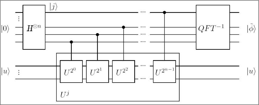
Figure 2. A quantum circuit for the face estimation procedure
The circuit begins by applying the n -qubit Hadamard transform H 0 n to the first quantum register, follows by the application of controlled U -operations on the second register, with U raised to successive power of two. This sequence maps
2 n -1 2 n -1
-
1 0) I U - Zl jU j u ) = iL e="j »-
- 2 j=0 2 j=0
2.
Apply the quantum oracle: U j Ag| jjU j W = -1 2- g e2'* |j)|u) 2 j =0 2 j =0
3.
Calculate the inverse quantum Fourier transform and measure the first register:
QFT "1 . хм , „
^ ф u)^ф
With ф = 0 ф .. ф this state may be rewritten in product from which is equivalent to the product representation (Eq. (29)). If ф is exactly expressed in n qubits the application of the inverse QFT to the first qubit register leads to the state ф = | ф 1 ... ф п ) , or a good estimator ф otherwise.
Computing QFT-1 can be seen as the actual phase estimation step .
|
Quantum Algorithm : Quantum phase estimation |
|
|
1. |
| 2 n -1 Create the equally weighted superposition: 0 u H j u ' ' 2 n2 м' |
A final measurement of the first register yields to the result ф or ф respectively. To estimate ф with k -bit accuracy and probability of success at least 1 — 6 , choose n = k + " log ( 2 + ^ ) | .
This algorithm, summarized below, computes the approximation ф to ф using O ( n 2 ) operations and one query to the controlled- U j oracle gate.
Even if the eigenvector u is unknown and cannot be prepared, running the phase estimation algorithm on an arbitrary state | ^ ) = g c^u) (written in terms of eigenstate | u )) yields a state g cu |ф^ |u ), where ф is a good approximation to ф . Assuming that n is chosen as specified above, the probability for measuring ф with k -bit accuracy is at least \cu |2 ( 1 — c).
Order-Finding and Other Applications
The order-finding problem reads as follows: for x, N e N, x < N, gcd (x, N) = 1, determine the least r eN, such that xr = 1mod N. It is believed to be a hard problem on classical computers. Let n = "log N| be the number of bits needed to specify N. The quantum algorithm for order-finding is just the phase estimation algorithm applied to the unitary operator U|y^ - |xy mod N with y e{0,1}n and | u) = 11), a superposition of eigenstates of U (for N < y < 2n — 1 , define xy mod N := y).
The entire sequence of controlled- U 2 l operations can be implemented efficiently using modular exponentiation : It is
In a first step modular multiplication is used to compute successively (by squaring) x2j modN from x2j—1 for all j = 1...t — 1. In a second step xz modN is calculated by multiplying the t terms(xz 2 modN)...(xz02 modN). On the basis of this procedure the construction of the quantum circuit computing U : |z^|y^ ^ |z^x2 modN is straightforward, using O(n3) gates in total.
To perform the phase estimation algorithm, an eigenstate of U with a nontrivial eigenvalue or a superposition of such eigenstates has to be prepared. The eigenstates of U are 1 r —1
Ius) -^g®— sk |xk modN , r k=o for 0 < s < r — 1. Since 1j4т gr_11 us } = Ц it is sufficient to choose | u) = 11) .
Now, applying the phase estimation algorithm on t = 2 n + 1 + | log ( 2 + 1/2c ) | qubits in the first register and a second quantum register prepared to |1) leads with a probability of a least (1 — e)/ r to an estimate of the phase ф ~ s/r with 2 n + 1 bits accuracy.
From this result, the order r can be calculated classically using an algorithm, known as the continued fraction expansion . It efficiently computes the nearest fraction of two bounded integers to φ , i.e. two integers s ', t ' with no common factor, such that s ' r ' = s/r . Under certain conditions this classical algorithm can fail, but there are other methods to circumvent this problem.
An application of the order-finding quantum subroutine is Shor’s factorization algorithm. Other problems which can be solved using the order-finding algorithm are period-finding and the discrete logarithm problem. These and some other problems can be considered in a more general context, which will be explained in the following two subsections.
|
Quantum Algorithm: Order-finding |
|
|
1. |
Create superposition: H ⊗ n 2 t -1 1 0я1 H →⊗ n 21 t 2 ∑2 - 1 1 j )| 1 } 2 j =0 |
|
2. |
Apply the black-box oracle U : 1 j ^1 k → x j k mod N , with x co-prime to N : U x , N 1 2 t -1 1 r -1 2 t -1 → 2 t 2 ∑ j x mod N ≈ 2 t 2г ∑ r -1 ∑2-1 e 2 π isj r 1 j )1 u s 2 j =0 2 r s =0 j =0 |
|
3. |
Calculate the inverse QFT of the first register and measure this: QFT - 1 r -1 M 1 → ∑ s r u s → s/r r j =0 |
Fourier Transform on Arbitrary Groups
The more general definition of the Fourier transforms FT on an arbitrary group G needs some background in algebra and in representation theory over finite groups.
Let G be a finite group of order N and f : G →с . The Fourier transform of f at the irreducible representation ρ of G (denoted f ˆ ( ρ ) ) is defined to be the d × d matrix
f(ρ) = dρ ∑ f (g)ρ(g) .
Remark . A representation ρ of a finite group G is a homomorphism ρ : G → GL ( V ) , where V is a с-vector space. The dimension of V is called the dimension of the representation ρ , denoted d . ρ is said to be irreducible, if no other subspaces W are G -invariant, i.e. ρ ( g ) W ⊆ W , ∀ g ∈ G , expect 0 and V . Up to isomorphism, a finite group has a finite number of irreducible representations. G denoted such a set of irreducible representations, which is a complete system of representatives of all isomorphism classes.
The collection of matrices f ( ρ ) is designated as the Fourier transform of f. Thus, the Fourier
ρ∈ G transform maps f into G matrices of varying dimensions which have totally ∑ d2 = G I entries. This means that the IGI complex numbers f (g) are mapped into IGI complex numbers organized into matrices. Furthermore, the Fourier transform is linear in f (f + f (p) = f (p) + f (p)) and f (p) is unitary for all p e G .
If G is a finite Abelian group, all irreducible representations have dimension one. Thus, the representations correspond to the | G | (irreducible) characters x : G ^ Cx of G . It is ( G , + ) — ( G , * ) . This is quite useful to simplify the notation by choosing an isomorphism g I—> % .
With the operation (x * X )(g) = X (g)* X (g) the set G of all characters of G is an Abelian group, called the dual group of G. Any value x(g) is a |G|th root of unity, i.e. x(g)G = 1 . For instance, if G = Zv then the group of characters is the set {x (j) = ^jk | j, k = 0...N -1} and the Fourier transform corresponds to the classical DFT. For G = Z^ the Fourier transform FTn corresponds to the Hadamard transform H 0n
.
By the structure theorem of infinite Abelian groups, G is isomorphic to products of cyclic groups Z of prime power order with addition modulo p. being the group operation i.e. G — Z x...x Z n . Any g e G i p1
can be written equivalently as (gj,...,gm ) , whereg± eZ^ . This naturally leads to the description of the characters g. e Z on G as the product of the characters Xpi on Z It is i pip
XG (g )=П XA gj=fp“ У , i=1
Remark . The following mapping is used: ( g,,..., gm )l— »П;”=1 X ? ( g i ) • With h = ( h v ..., h m )
and qt := N/p . Note that x (g) = X (h). With Eq. (30) the Fourier transform of a function f: G > C may be written as f (h) = —J= У f (g)X (h), with h e G. Using the conventional notation, the QFT on v n g- x yx ’ an Abelian group G acts on the basis states as follows: QFTG |h) = А- У x (h)| g).
I G | ge G
The Hidden Subgroup Problem
Nearly all know problems that have a quantum algorithm which provides an exponential speedup over the best known classical algorithm can be formulated as a hidden subgroup problem (HSP). Problem instances are for example order-finding, period-finding and discrete logarithm. The HSP is: Let G be a finitely generated group, H < G a subgroup, X a finite set and f : G ^ X a function such that f is constant on cosets g = g H e G/ H and takes distinct values on distinct cosets, i.e. f ( gt ) ^ f ( g2 ) for gt ^ g2 . Find a generating set for H .
Definite H° : = { g e G : x ( h ) = 1, V h e H } , also called the annihilator group of H . Note that H ° is equivalent to the subgroup H 1 = { x : H c ker x } , which in turn is isomorphic to the dual of H 1 = { x : H c ker x } . The algorithm for solving the HSP uses the following two properties of the Fourier transform over G.
V k


l
7

V k

The superposition state, uniform on H , is mapped to H :
H
QFT
Zl h ЛH heH \ G

k e H
Using this, it follows for a coset state V T H Z g h :
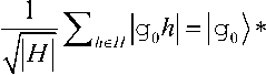

Z he, №
QFT GH , EQ (32) —

( Z g .G X g ( g o )| g) ) - ( Z ke h W )

Z k . H X ( g 0 )l k)
So, the QFT takes a coset state to the annihilator group states of the corresponding subgroup where the coset is encoded in the phase of the basis vectors.
Assume that G is Abelian. A hybrid algorithm to solve the Abelian HSP consists of the following quantum subroutine:
|
Quantum Algorithm : Abelian HSP |
||
|
1. |
Create a random coset state: QFTCt ® I 1 U f 10>|0> -> У Zl g)|0 )P- G g eG ^ |
M 2 r— Zl g) f (g))— /77 Z |g o h) ' G g eG J H heH |
|
2. |
Fourier sample the coset state: 1 QFT G H V H , Z H |gJ v g i |
■ Z X k ( g o)l^-- k e H k e H |
M denotes the measurement of the i-th quantum register. The process of computing the Fourier transform over a group G and measuring subsequently is also called Fourier sampling. After applying M , it is sufficient to observe the first register. The last measurement results in one out of GH elements H kz. e H with probability . Repeating this process t = poly (log |G|) times leads to a set of element which describe the X e H1. Thus, H can be classically computed as the intersection of the kernels of Xi:H = A^oker Xi.
The efficient quantum circuit for the Abelian HSP is shown in Fig. 3.
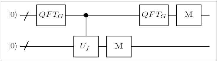
Figure 3. A quantum circuit for the Abelian HSP
Generalizations of the Abelian HSP quantum algorithm to the non-Abelian case have been attempted by many authors, unfortunately only with limited success. Up to now, the problem is still open, except for only a few particular instances.
A coarse outline on QFT-based algorithms
Table 2 shows an overview on problems efficiently solvable by means of quantum algorithm based on the QFT.
Table 2. The quantum Fourier transform and algorithms based on it.
|
Problem |
Runtime |
|
(discrete) QFT |
© ( n 2 ) or O ( n log n ) resp. |
|
Deutsch † |
1 oracle query |
|
Deutsch-Jozsa † |
1 oracle query |
|
Bernstein-Vazirani |
1 oracle query |
|
Simon † |
O ( n ) repet. with 1 oracle query each |
|
Period-finding † f with f ( x + r ) = f ( x ) , x , r e N 0,0 < r < 2 n , a periodic function, output r! |
1 oracle query, O ( n 2) operations |
|
Phase estimation |
O ( n 2 ) +1 oracle query |
|
Order-finding † |
0 ( n 1) |
|
Factoring † |
O ( n 3) operations, O ( n1 log n log log n ) |
|
Discrete logarithm † given: a, b = as mod N determine s |
polyn. time QA |
|
Hidden linear function problems † |
polyn. time QA |
|
Abelian stabilizer † |
polyn. time QA |
|
Shifted Legendre symbol problem and variants |
polyn. time QA |
|
Computing orders of finite solvable groups |
polyn. time QA |
|
Decomposing Finite Abelian Groups |
polyn. time QA |
|
Pell’s Equation & Principal Ideal Problem |
polyn. time QA |
Problems marked with † are special instances of the HSP. The parameter n is the input length of the given problem.
The following explanations and annotations refer to single problems given below in the table.
Abelian group stabilizer problem: Let G be an Abelian group acting on a set X. Find the stabilizer G x : = { g e G g • x = x } for x e X .
Decomposing finite Abelian groups: Any finite Abelian group G is isomorphic to a product of cyclic groups. Find such a decomposition. For many groups no classical algorithm is known which performs this task efficiently.
The quantum algorithm mainly uses the quantum algorithm for HSP to solve a partial problem. The rest is done classically.
An application of this algorithm is the efficient computing of class numbers (assuming the generalized Riemann Hypothesis).
Deutsch’s problem: Determine whether a black-box binary function f : {^’^ ^ {^’^ is constant (or balanced).
k
Hidden linear function problem: Let f be a function for an arbitrary range S with
f (xx,...,xk) = h(xx+ax^ +...+axk) г г v u a ^z „ 1
-
1 k 1 2 2 k k for a function h with period q and i . Recover the values of
all the a i ( mod q ) form an oracle for f. This problem is an instance of the HSP.
Inner product problem (Bernstein-Vazirani): For a E
{0,1}}
. t fa : { 0,1 } n ^{ 0,1 } . . _ .
let a be defined
by f a ( x ) = a • x
Calculate a. This problem is not directly an instance of the HSP. Nevertheless, Fourier
sampling helps finding a solution, too.
Orders of finite solvable groups: The problem is described.
Pell s Equation: Given a positive non-square integer d, Pell s equation is x dy . Find integer so
d lutions. The quantum algorithm calculates the regulator of the ring , which is a closely related prob lem. The quantum step in this algorithm is a procedure to efficiently approximate the irrational period S of a function in time polynomial inlnS .
a gQ)(Vd)
Principal ideal problem: Given an ideal I, determine (if existing) an such
I = aZl dd\ that . The algorithm reduces to a discrete log type problem.
f
Shifted Legendre symbol problem (SLSP): Given a function s and
an
odd prime p
such
f (x) = (x±^) x E % that s p , for all p , find s! Variants of this problem are the shifted Jacobi symbol problem and the shifted version of the quadratic character x over finite fields q (shifted quadratic character problem). The classical complexities of these problems are unknown.
. a ^ { 0,1 } n Д f : { 0,1 } n ^ { 0,1 } n . V W f ( x ® a ) = f ( x )
Simon’s problem: Let ( } and ( } ( j a function with v v 7 ( ш : bitwise XOR). Calculate a. Simon’s problem was the first that was shown to have an expected polynomial time quantum algorithm but no polynomial time randomizes algorithm. Brassard and Hoyer an exact quantum polynomial-time algorithm to solve this problem.
Two other transformations which can be recovered from the DFT are the discrete cosine transformation and the discrete sine transformation. Klappenecker and Rotteler show that both transformations of
size N x N
O ( N log N )
and types I-IV can be realized in
O ( log 2 N )
operations on a quantum computer instead of
on a classical computer. Another class of unitary transforms, the wavelet transforms, are
efficiently implementable on a quantum computer. For a certain wavelet transform, a quantum algorithm is designed using the QFT.
Quantum Search Algorithms
Search problems are well-known and intensively investigated in computer science. Generally spoken, a search problem is to find one or more elements in a (finite or infinite, structured or unstructured) search space, which meet certain properties.
Suppose, a large database contains N 1 items in a random order. On a classical computer it takes (^) comparisons to determine the items searched for. However, there is a quantum search algorithm, also
O ( VN )
called Grover’s algorithm, which required only operations.
Grover’s algorithm is optimal for unstructured search problems.
Also in some cases of structured search spaces quantum algorithms can do better than classical as demonstrated by Hogg’s algorithm for 1-SAT and highly constrained k-SAT.
Grover’s Algorithm
It is assumed that N = 2 . The database is represented by a function f which takes as input an integer x ,0 < x < N - 1 (the database index), with f ( x ) if x is a solution to the search problem and
f ( x ) ^ otherwise. Let ^ be the set of solutions, i.e.,
L = {x^f (x) = 1, x e
and
M = M
the number of solutions. Furthermore, let be ф=. N-M-
N
V N - M
21 x) 1в= x^£ ,
= 21 x)
M xec and
i a +, M i e = 4= N -i x > ■
1 ' V n'p Nn 2' '
This algorithm works on two quantum registers xy , where x is the index register and single ancilla qubit. Let U a be the black-box which computes f. Then applied
is a
to the
state
, the oracle “marks” all solutions by shifting the phase of each solution. Ignoring the
single qubit register, the action of U a may be written as
or U . = I - 2| вв
.
Geometrically, U a induces a reflection about the vector . in the plane defined by . and' в . Another important operation, denoted with ^ ф , is the so-called inversion about the mean:
иф = H 0 n ( 2|0>(0| - 1 ) H 0 n = 2 | фф | - 1 .
Applying Uф to a general state | . = 2* a | k ) leads to
UO) = 2|^| a )-I a ) = 2 2 A\k) - 2 a^ = 2 ( 2 A - ak )| k)
k
k
k
using state
+2, ak = 2nAA A = 2 ak
-
2 k , where 2 k is the mean of the amplitude. Thus, the
amplitudes are transformed as ^ф ' a k ^^ a k , i.e., the coefficient of '' is reflected about the mean value of the amplitude. In other words, ^ф is a reflection about the vector ф in the spanned by ' . and ' в
The combination of both operator U a and ф leads to the Grover operator, defined to be Ug = и ф и . =- H •’' (2|0)(0| - 1 ) H»' ( 2| вв - 1 )
(see Fig. 4).
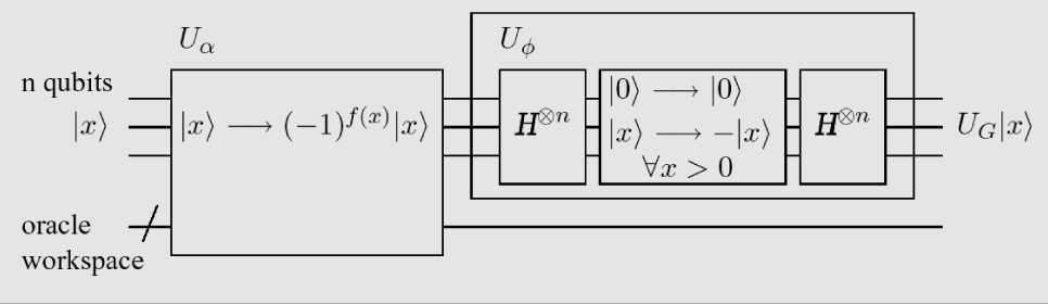
Figure 4. A quantum circuit for the Grover operator
Thus, the product of the two reflections U and U is a rotation in the two-dimensional subspace spanned by | O) and | в rotating the space by an angle в, defined by sin в/2 = ^M (N , as shown in Fig.5.
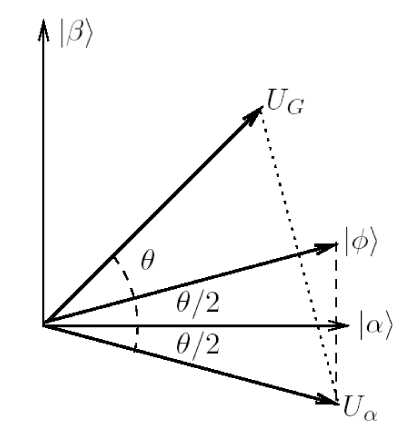
Figure 5. Geometric visualization of the single step of the Grover iteration
Repeating the Grover operator T — П 4 ^ N/M = O (^ N/M ) times rotated the initial system state ф close to | в) . Observation of the state I the computational basis yields a solution to the search problem with probability at least p > 1/2 . When M N th this probability is at least 1 - M /N , that is nearly 1.
Figure 6 illustrates the entire quantum search algorithm. It should be mentioned that the quantum search algorithm is optimal, i.e. no quantum algorithm can perform the task of searching N items using fewer than q ( V N ) accesses to the search oracle.
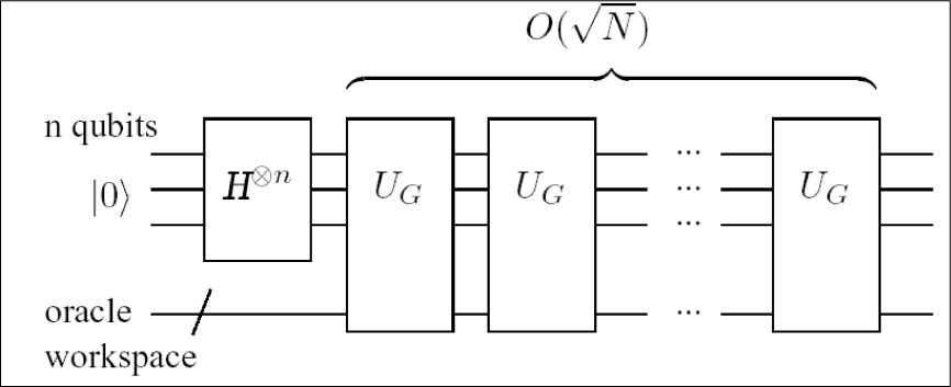
Figure 6. Quantum circuit for the QSA
A concluding note: In the basis { a^ , | в } the Grover operator may also be written as
Ug =
6 cos 0 v sin 0
— sin 0 cos 0 ,
where 0 < 0 < п/ 2 , assuming without limitation that M < N /2. Its eigenvalues are e1 i 0 . If it is not known whether M < N /2, this can be achieved for certain by adding a single qubit to the search index, doubling the number of items to be searched to 2 N . A new augmented oracle ensured that only those items are marked which are solutions and whose extra bit is set to zero.
Remark . A generalization of the Grover iteration to boost the probability of measuring a solution state is called amplitude amplification. According to Gruska, there are at least two (only slightly different) methods which meet this condition, one proposed by Grover, the other by Brassard et al. The most general version of a Grover operator is presented by Biham at al. All methods have in common, that they use an arbitrary unitary transformation U instead of the Hadamard transformation H 0 n as in the original Grover operator (Eq. (1.7)). The following transformation might be deemed as the generalized Grover operator :
Ug = —UIeU-1 If , where If = I — (1 — eв )| ^(sl is a rotation of a fixed basis state |s) by an angle в and Iy = ^^ e'^f(x) | x^x | is a rotation by an arbitrary phase 4.
Quantum Counting: Combining Grover Operator and Phase Estimation.
Provided that M is known, Grover’s algorithm can be applied as described above. If M is not known in advance, it can be determined by applying the phase estimation algorithm to the Grover operator U , estimating one of its phases ± 0 .
Figure 7 shows a quantum circuit for performing approximate quantum counting.
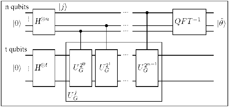
Figure 7. Circuit for the quantum counting algorithm
An application of the phase estimation procedure to estimate the eigenvalues of the Grover operator U G which enables to determine the number of solutions M to the search problem. The first register contains n qubits and the second register contains t qubits, sufficient to implement Grover’s operator on the augmented search space of size 2N . The state of the second register is initialized to ^ | x^ by H ® n .
x
But this is a superposition of the two eighenvectors of Ug with corresponding eighenvalues e i and e (2 n -9 ) . Therefore applying the phase estimation procedure, results in the estimate for 6 or 2 n - 6 which is equivalent to the estimate for 6 ( sin 2 ( 6 /2) ) = sin 2 ((2 n — 6 )/2) From the equation sin 2 ( 6 2 ) = M 2^ N and the estimate for 6 it follows as estimate for the number of solutions M .
Remark. The search space is expanded to 2 N to ensure that M < N /2 . As already described above this is done by adding a single qubit to the search space.
Further analysis shows, the error in this estimate for M is less than (V 2 MN + - N ) 2 k , provided that 6 has a k -bit accuracy. Summarizing, the algorithm requires O (V N ) oracle calls to estimate M to high accuracy. Finding a solution to a search problem when M is unknown requires to apply both algorithms, first the quantum counting and then the quantum search algorithm. Errors arisen in the estimate for 6 and M affect the total probability to find a solution to the search problem. However, the probability can be increased close to 1 by a few repetitions of the combined counting-search algorithm.
Counting the number of solutions and, consequently, determining the solvability of a search problem has many applications, including decision variants of NP-complete problems.
Applications of Grover’s Algorithm
The quantum search algorithm or at least its main operator can be applied to solve many kinds of search problems. Table 3 presents a survey of these problems. Some of them are now described briefly.
Table 3. Algorithms based on quantum searching.
|
Problem |
Runtime |
|
Quantum database search (Grover’s algorithm) |
O ( V N ) quadratic speedup |
|
Quantum counting |
о (V N ) |
|
Scheduling problem |
O ( N 34 log N ) |
|
Minimum-finding |
o (V N ) |
|
Database retrieval |
N / 2 + O ( V N ) |
|
String matching |
O (v n log ^ log m + V m log 2 m ) |
|
Weighing matrix problem |
2 oracle queries |
|
Element distinctness Collision funding Claw finding Triangle-finding |
comparison complexity always better than classical |
Claw finding: Given two functions f : X ^ Z and g : Y ^ Z , find a pair ( x , y ) е X x Y such that f ( x ) = g ( y ) .
Collisions finding: Given a function f : X ^ Y , find two different X j, x 2 ( X j ^ x 2), such that f ( X j ) = f ( x 2) under the promise that such a pair exists.
Database retrieval: Given a quantum oracle which returns | k , y ® X^ on an n +1 qubit query | k , y ^ , the problem is to obtain all N = 2 n bits of Xk .
Element distinctness: given a function f : X ^ Y , decide whether f maps different x е X to different y е Y .
Minimum-finding : Let T [ 0... N — 1 ] be an unsorted table of N (distinct) items. Find the index y of an item such that T [ y ] is minimal.
Scheduling problem: Given two unsorted lists of length N each. Find the (promised) single common entry. The complexity is measured in quantum memory accesses and accesses to each list.
String matching: Determine whether a given pattern p of length m occurs in a given text t of length n . The algorithm combines quantum searching algorithms with deterministic sampling, a technique from parallel string matching. Grover’s search algorithm is applied twice in conjunction with a certain oracle in each step.
G ( V, E )
Triangle-finding: Given an undirected graph v ' , find distinct vertices , , such that
( a , b ) , ( a , c ) , ( b , c ) е E
.
_ . , . • , W ( n , k ) • , •
Weighing matrix problem: Let M be a weighing matrix.
D _ , . „ . • M е { - 1,0, + 1 } • M • MT = k • J p
Remark. A matrix is called a weighing matrix, iff n for some
.
A set of n functions termine s.
n} ^ {-1,0,+1} for
n } is defined by fs (z) : si^sl . De-
Quantum Search and NP Problems
Solving problems in the complexity class NP may also be speed up using quantum search. The entire search space of the problem (e.g. orderings graph vertices) is represented by a string of qubits. This strings has to be read as defined by the problem specifications (e.g. the string consists of blocks of the same length storing as index of a single vertex). In order to apply the quantum search algorithm, the oracle which depends on the problem instance must be designed and implemented. It marks those qubit strings which represent a solution. As the verification of whether a potential solution meets the requirements is much easier than the problem itself, even on a classical computer, it is sufficient to convert the classical circuit to a reversible circuit. Now, this circuit can be implemented on a quantum computer. Thus, the quantum counting algorithm which determines whether or not a solution to the search problem exists requires the square root of the number of operations that the classical “brute-force” algorithm requires. Roughly speaking, the complexity
O ( 2 y ( n ) ) O ( 2 e ( n^ 2 ) n . . . . .
changes from to , where y is some polynomial in n . Nonetheless, the complexity is still exponential and in the sense of complexity theory these problems are not efficiently solved.
Hogg’s Algorithm
Certain structured combinatorial search problems can be solved effectively on a quantum computer as well, even outperforming the best classical heuristics. Hogg introduced a quantum search algorithm for 1-SAT and highly constrained k -SAT.
The satisfiability problem (SAT). A satisfiability problem (SAT) consists of a logical formula in n variables v ,..., vn and the requirement to find an assignment a = ( ax,...,an ) e { 0,1 } n for the variables that makes the formula true. For k -SAT the formula is given as a conjunction of m clauses, where each clause is a disjunction of k literals v. or v respectively with i e { 1... n } . Obviously there are N = 2 n possible assignments for a given assignment are called conflicts. Let c ( a ) denote the number of conflicts for assignment a. A k-SAT problem is called maximally constrained if the formula has the largest possible number of clauses for which a solution still exists. Thus, any conceivable additional clause will prevent the satisfiability of the formula. For k > 3 the satisfiability problem is NP-complete and in general, the computational costs grow exponentially with the number of variables n . For k = 1, k = 2 , and some k-SAT problems with a certain problem structure, there are classical algorithms which require only O ( n ) search steps , that is, the number of sequentially examined assignments. Also, quantum algorithms can exploit the structure of these problems to improve the general quantum search (ignoring any problem structure) as perform better than classical algorithms.
Hogg’s quantum algorithm for 1-SAT . Hogg’s quantum algorithm for 1-SAT primarily requires n qubits, one for each variable. A basis state specifies the value assigned to each variable and consequently, assignments and basis state correspond directly to ach other. Information about the particular problem to be solved is accessible by a special diagonal matrix R (of dimension 2 n x 2 n ), where
R. = ' "“ ' (35)
is the matrix entry at position ( a,a ). Thus, the problem description is entirely encoded in this input matrix by the number of conflicts in all 2 n possible assignments to the given logical formula. For the moment it is assumed that such a matrix can be implemented efficiently. Further implementation details will be given in the next paragraph.
Figure 8 exemplifies the input matrix R for a 1-SAT problem with n = 3 variables.
/10 0
0 г 0
0 0 i
0 0 0
0 0 0
0 0 0
0 0 0
\ 0 0 0
0 0 0
0 00
0 00
-10 0
0 г 0
00-1
0 0 0
0 0 0
о 0 \ о 0
о 0
о 0
о 0
о 0
-1 0
0 -i /
Figure 8. Input matrix for he local formula f ( v , v 2, v 3) = v л v 2 л v3 . The matrix has diagonal coefficients (ic (000) ,..., ic (111) ). Off instance the assignment a=101 ( v = true, v 2 = false, v 3 = true ) makes two clauses false, i.e. c(101)=2 and i2= -1
Furthermore, let U be the matrix defined by
U rs
2 - n / 2
e
in ( n - m
M 4
(- i )
d ( r , s )
where d ( r , s ) is the Hamming distance between two assignments r and s , viewed as bit strings. U is independent f the problem and its logical formula. The first step of the quantum algorithm is the preparation of an unbiased, i.e. equally weighted, superposition. An already demonstrated, this is achieved by applying the Hadamard gate on the n qubits ( H 0 n ) initially is state 10^ .
Let | ^ ) denote the resulting quantum state. Then, applying R and U to | y ) gives I ф = UR I T .
It was proven that the final quantum state is the equally weighted superposition of all assignments a with c ( a ) = 0 conflicts. Thus, considering a soluble 1-SAT problem, a final measurement will lead with equal probability to one of the 2 n - m solutions. If there is no solution of the problem, the measurement will return a wrong result. Hence, finally the resulting assignment has to be verified.
Implementation. The matrices R and U have to be decomposed into elementary quantum gates to build a practical and implementable algorithm. The operation R can be performed using a reversible (quantum) version of the classical algorithm to count the number of conflicts of a 1-SAT formula and a technique to adjust the phases which are powers of . Therefore, two ancillary qubits are necessary which are prepared in the superposition
I T= 1 (1 °- -101)-1 10 +' 111) ) .
where the local phases correspond to the four possible values of R for any assignment a . As suggested by Hogg, the superposition | T can be constructed by applying H on qubit 1 and R ( 3/4 n ) on qubit 0, both of the qubits being initially prepared to |1) . Then, the reversible operation
F: | a, x^ ^ | a, x + c ( a ) mod 4^
acts on | y , T as follows
| y, T}^ 2-n/2 £ 0(a) | a) |T) a performing the required operation R. To see this, further intermediate calculation steps are necessary. Note that after applying F, the ancillary qubits reappear in the original superposition form and can therefore be dropped, since they do not influence U. In a single application of F, c (a ) is evaluated once.
The matrix U can be implemented in terms of two simpler matrices H 0 n and Г , where Г is diagonal with Г aa = aa. . Here | a | is the number of 1-bits in the string of assignment a . Using this definition, it is U = H 0 n Г H 0 n . For implementing Г , Hogg suggests to use similar procedures to those for the implementation of the matrix R , using a quantum routine for counting the number of 1-bits in each assignment instead of the number of conflicts. Thus, the elements of the matrix Г can be computed easily and the operation U is efficiently computable in O ( n ) bit operations: 2 n Hadamard gates plus another C • n elementary single qubit gates, with a constant C > 1, fir the computation of Г (to give a rough estimation). It is shown as a result of the GP evolution of a 1-SAT quantum algorithm that U = R ( 3/4 n ) 0 n
, and consequently it can be implemented even more efficiently by n elementary rotation gates. Once again, Hogg’s algorithm consists of the following steps:
|
Quantum Algorithm : 1-SAT / maximally constrained k-SAT |
|
|
1. |
Apply H ® n on| 0^. |
|
2. |
Compute the number of conflicts with the constraints (clauses) of the problem into the phases by applying the input gate R . |
|
3. |
Applying U = H ® n Г H ® n results in an equally weighted superposition of solution states. |
An experimental implementation of Hogg’s 1-SAT algorithm for logical formulas in three variables was demonstrated.
Performance. The matrix operations and the initialization of | ^ contribute O ( n ) bit operations to the overall costs. Evaluating the number of conflicts results in costs of O ( m ) for a k-SAT problem with m clauses. In total the costs of the quantum algorithm amount to O ( n + m ) . This corresponds to the costs of a single search step of a classical search algorithm which is based on examinations of neighbors of assignments. While the quantum algorithm examines all assignments in a single step, the best (local search based) classical algorithm needs O ( n ) search steps.
A slide modification of Hogg’s algorithm for 1-SAT can also be applied to maximally and highly constrained k -SAT problems for arbitrary k to find a solution with high probability in a single step. For all 1-SAT and also maximally constrained 2-SAT problems, Hogg’s algorithm finds a solution with probability one. Thus, an incorrect result definitely indicates the problem is not soluble.
Note that a comparison of Hogg’s algorithm with any classical algorithms according to the number of search steps is only permissible, if the classical algorithms are based on local search, especially on the examination of the number of conflicts. Otherwise, the comparison must be based on a more fundamental measure. Local search is not always the best solution. For instance, it is unreasonable to solve 1-SAT using local search since it is trivial to find an assignment satisfying the given Boolean formula in O ( m ) .
Quantum Simulation
The third class of quantum algorithms consists of those algorithms which simulate quantum mechanical systems. Commonly, the problem of simulating a quantum system is classically (at least) as difficult as simulating a quantum computer. This is due to the exponential growth of the Hilbert space which comprises the quantum states of the system. Therefore, simulation of quantum systems by classical computers is possible, but in general only very inefficiently. A quantum computer can perform the simulation of some dynamical systems much more efficiently, but unfortunately not all information from the simulation is accessible. The simulation leads inevitable to a final measurement collapsing the usually superimposed simulation state into a definite basis state. Nevertheless, quantum simulation seems to be an important application of quantum computers.
A rough outline of the quantum simulation algorithm is presented now. Further reading matter are the original papers dealing with the simulation of quantum physical systems on a quantum computer.
Simulating a quantum system means “predicting” the state of the system at some time t (and/or position) as accurately as possible given the initial system state. Simulation is mainly based on solving differential equations. Unfortunately, the number of differential equations increases exponentially with the dimension of the system to be simulated. The quantum counterpart to the simple differential equation dy/dt = f (y) in classical simulations is id|^}/dt = H^^ for a Hamiltonian H. Its solution for a timeindependent H is | ф(t)^ = e~iHt | ф(0)/ . However, e~iHt is usually difficult to compute. High order solutions are possible especially for those Hamiltonians which can be written as sums over local interactions: H = ^Lk_xHk , acting on a n-dimensional system, L = poly(n) where each Hamiltonian HK acts on a small subsystem. Now, the single terms e-iHt are much easier to approximate by means of quantum circuits than e- iHt. How to calculate e- iHt from e-iHkt ?
In general e iHt ^ ^^ e iH k t because of ^ H, Hk J ^ 0 . Instead, approximate e iHt with e.g.
e ( A + B )A t = e iA A t /2 eB%и A t /2 + о ( ^ t з ) .
This and other approximations are derived from the Trotter formula lim ( e V) ” = e l ( A + B ) t . n ^to
Now, let the n-qubit state | V } approximate the system. Assume further, that the operators e"iHkAt have l (У Hk )a efficient quantum circuit approximations. Then, the approximation of e k can be efficiently implemented by a quantum circuit U . With it, the quantum simulation algorithm can be formulated as follows:
|
Quantum Algorithm : Quantum simulation algorithm |
||
|
1. |
Initialization: | ^ ) (initial system state at time t = 0), j = 0 ; |
|
|
2. |
Iterative evolution: do | yj+x ^ = UM | ^ . ^; j = j + 1 ; until j A t > t^ |
|
|
3. |
Output: |
V ( t f )) = ^-) |
Speedup Limits for Quantum Algorithms
This section summarizes some theoretical results about the limitations of quantum computing. The methodologies to prove lower bounds for the complexity and the speedup of quantum algorithms are not the subject matter, but they can be read up in the given literature.
An interesting result on limitations of quantum algorithm refers to black-box algorithms. Many quantum algorithms use oracle or black-box algorithm. Accessing the black-box can be thought of as a special subroutine call or query whose invocation only costs unit time. Speaking more formally, let X = ( x 0,..., xN 4) be a such an oracle, containing N Boolean variables x e { 0,1 } . On input i the oracle returns xt . A property f of X which is any Boolean function f : { 0,1 } N ^ { 0,1 } is only determinable by oracle queries. The complexity of a black-box algorithm is usually rated by the number of queries necessary to compute the property. Then, Beals et al. prove that black-box quantum algorithm for which no inner structure is known, i.e., for which no promises are made restricting the function. Then, the function is said to be total. Can achieve maximally a polynomial speedup compared to probabilistic and deterministic classical algorithm. In addition, they specify exact bounds for the (worst case) quantum complexity of AND, OR, PARITY and MAJORITY for different error models (assuming exact -, Las Vegas – and Monte-Carlo algorithms). For the exact setting (the algorithm returns the correct result with certainty) the quantum complexities are N for OR and AND, N/2 for PARITY and ® ( N ) for MAJORITY. The bound for the parity problem was independently obtained by Farhi et al.
As shown by Buhrman at al. the following problems cannot be solved more efficiently on a quantum computer:
Parity-collision problem: Given a function f : X ^ Y , find the parity of the cardinality of the set { ( xx , x 2) e X x X|x t< x 2 л f ( xx ) = f ( x 2) } .
No-Collision problem: Given a function f : X ^ Y , find an element x е X that is not involved in a collision, i.e., f -1 ( f ( x ) ) = { x } .
No-range problem: Given a function f : X ^ Y , find an element y е Y such that y £ f ( X ) .
Hoyer at al. determined the quantum complexity for further problems.
Ordered searching: Given a sorted list of N numbers ( x 0, X j,..., xN 4) , x < x /+1 and a number y < xN 4 , find the minimal index i such that y < x z.. This problem can be regarded as a non-Boolean promise problem. The best known quantum lower bound is 1/ n ( In ( N ) - 1 ) queries. A quantum algorithm using log3 ( N ) + O ( 1 ) « 0.631log2 ( N ) queries is presented. A slightly better algorithm ( 0.526log2 ( N ) queries) is given.
Sorting: Given a list of numbers ( x 0, X j,..., xN _J , output a permutation ст on the index set such that the list ( xa °, xa ,...,xa ) is in non-decreasing order. The quantum lower bound for this problem is given by Q ( N log N ) binary comparisons.
Element distinctness: Given a list of numbers (x0, Xj,..., xN_j) . Decide whether they are all distinct. The problem has a quantum lower bound of
q ( 4N log N ) binary
comparisons.
References Examples of quantum computing toolkit: Kronecker product and quantum Fourier transformations in quantum algorithms
- Gruska J. Quantum computing. - Advanced Topics in Computer Science Series, McGraw-Hill Companies, London. - 1999.
- Nielsen M.A. and Chuang I.L. Quantum computation and quantum information. - Cambridge University Press, Cambridge, Englandю - 2000.
- Hirvensalo M. Quantum computing. - Natural Computing Series, Springer-Verlag, Berlinю - 2001.
- Hardy Y. and Steeb W.-H. Classical and quantum computing with C and Java Simulations. - Birkhauser Verlag, Basel. - 2001.
- Hirota O. The foundation of quantum information science: Approach to quantum computer (in Japanese). - Japan. - 2002.
