Experimental determination of vibration conductivity by rocket sled structural elements in high-speed track tests of aircraft equipment

Author: Astakhov S.A., Biryukov V.I., Kataev A.V.
Journal: Siberian Aerospace Journal @vestnik-sibsau-en
Section: Aviation and spacecraft engineering
Article in issue: 1 vol.24, 2023.
Free access
The development of new ballistic-type aircraft is characterized primarily by improved aerodynamic characteristics and higher speed limits. Ground track testing of aviation and rocket technology is a stage whose task is to confirm the efficiency and effectiveness of new developments. Track tests make it possible to simulate real loads, they are simpler and much cheaper than flight tests. Experimental installation "Rocket rail track 3500" of Scientific Test Range of Aviation Systems named after L. K. Safronov is constantly being upgraded in order to conduct track tests of products at a speed greater than 3M. The experimental setup includes a two-rail track, made on a special foundation, which excludes unacceptable rail deflection with a mass of up to 3000 kg. The rail track has an acceleration section with an angle of attack 2500 m long and a deceleration section. A tray filled with water is made on the braking section between the track rails. It is designed for hydrodynamic braking to a complete stop of the rocket sled with stored equipment. The movable rocket track sled is made of a massive steel plate to which three cross beams are welded. The front and rear beams end with axles on which sliding supports are pivotally mounted. On the rear and middle beams there are lodgements for fastening rocket engines of solid fuel. Depending on the required test speed, from one to five motors can be placed on the cradles. The test object is usually mounted on the front and middle beams along the axis of the sled and fixed in a cantilever, with the head part extended forward. The design of the supports – shoes is made to encircle the rail head in such a way that it provides sliding contact along the upper plane of the rail head, and in the event of a lifting force exceeding the weight of the sled at high speeds, it keeps the structure from free flight by contacting the lower surface of the rail head. Track high-speed tests of special equipment objects are always accompanied by intense vibration and shock effects of structural elements. Due to the desire to conduct track testing of products at a faster rate, it becomes necessary to reduce the level of dynamic loads and eliminate resonant interactions. The article presents an algorithm and methodology for statistical processing of random signals of three-axis vibration acceleration sensors installed on the shoes of the rocket track sled and on the fairing of the test object. Due to the placement of registration data storage devices on the sled, experimental vibration data were stored when testing the product at a speed of more than 1M. The autocorrelation functions of the signals of vibration accelerations of sensors placed on various elements of the rocket sled, the functions of mutual correlation of the corresponding signals, the density of the amplitude spectra, the density of the power spectra and the transfer functions that characterize the dynamic conductivity of vibrations from the shoes sliding along the rail guides to the test object were determined.
Ground tests, rail track, rocket sled, vibration, power spectrum density, correlation, transfer functions
Short address: https://sciup.org/148329673
IDR: 148329673 | UDC: 629.7:629.018 | DOI: 10.31772/2712-8970-2023-24-1-44-63
Text of the scientific article Experimental determination of vibration conductivity by rocket sled structural elements in high-speed track tests of aircraft equipment
Under accelerated movement, the slippers of the rocket sled experience shock disturbances and vibrations due to contact with the butt gaps of the rails, as well as due to the geometric irregularities of the rail surfaces. External disturbances that also affect the structure of the sled are vibrations generated by pressure pulsations in the engine combustion chamber and acoustic combustion noise. In addition, the source of vibrations is a purely non-stationary aerodynamic flow around the structural elements of the sled with the test object by the oncoming air flow. There are other sources of vibration as well. Experimental and theoretical study of vibration and shock effects on the track sled structure with test objects under conditions of the existing rail track is an urgent and significant task.
Any product that has mass and elasticity, loaded with body forces and moments, is a dynamic oscillatory system with an infinite number of degrees of freedom. To analyze the oscillations of such a system, the d'Alembert method is often used, in which the differential equations describing the equilibrium of the system, instead of body forces, use equivalent inertia forces. Thus, differential equations of free vibrations of an elastic body are obtained. The solution of these equations is presented as the product of coordinate functions and time functions that change according to a harmonic law [1–6]. In this case, the coordinate functions are modes of free oscillations, and the time dependences describe the motion as principal coordinates. Then the eigenoscillations of the dynamic system are modeled as the sum of the products of various modes of eigenoscillations and the principal coordinates. To study the forms of free oscillations, a boundary value problem is formulated in the form of a system of differential equations with zero right-hand sides and homogeneous boundary conditions, where the frequency of the system natural oscillations is the unknown. The design of the sled is presented in the form of a connected system of beams (plates, rods, pipes, etc.), which have bending and torsion rigidity. We make the assumption that the deformations are small, and then the theory of bending and torsion of beams in a linear formulation is applicable [1 –5].
When analyzing the vibration loading of products placed on track sleds for ground tests, approximations are often used in which a complex real system is replaced by a conditional system with lumped parameters having equivalent mass and elasticity [5–10]. The structural elements of the rocket sled 33AB-NO505 No. 2, designed at the enterprise, are: a track sled frame with hinged slippers and assemblies for accommodating solid propellant rocket engines (SPRE) and the test object itself [11]. The components and the rocket sled itself are characterized by mass (equivalent mass m ), mechanical rigidity (elasticity) k (N/m), and resonant frequency (ω 0 – circular frequencies of natural oscillations). The test object is placed on a sled with a cylindrical part with a fairing moved forward and fixed on the cantilever. An image of the design of a rocket track sled is shown in fig. 1.
The oscillatory movement of any component of the track sled of a system with one degree of freedom is due to the difference between the external exciting force P 0 sin ωt and the sum of the inertia, elasticity and damping forces, i.e.
x + 280ю0 x + «2 x = ®2 — sin mt, (1) 00 0 0k here ω0 – circular frequency of natural oscillations of the system; δ0 is a parameter proportional to the damping coefficient.
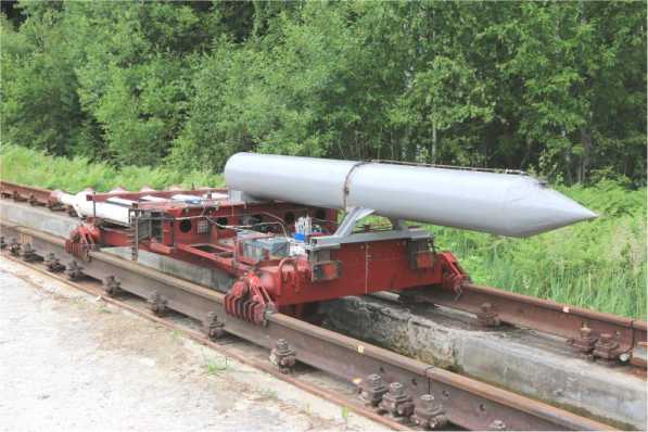
Рис. 1. Фотография трековой двухрельсовой каретки 33АВ-НО505 № 2 с башмаками для скольжения по рельсам и моделью объекта испытания. Связка из пяти РДТТ жестко закреплена в задней части каретки
Fig. 1. Photo of a track double-rail sled 33AB-NO505 No. 2 with slippers for sliding along the rails and a model of the test object. A bundle of five solid propellant rocket motors is rigidly fixed at the rear of the sled
For free oscillations in the absence of damping and initial conditions x ( 0 ) = х ( 0 ) = 0; x ( 0 ) = v , sinusoidal oscillations are realized with natural frequency and vibration amplitude А = v / ω 0
х = ( v / o 0 ) sin o 0 1 . (2)
For forced oscillations, the solution of equation (1) can be represented as the sum of homogeneous and particular solutions х = (v / o0 )e 50°0t sin(o01 — ф0) + (вP0 / k)sin (ot - ф).
Here φ is the initial phase of the driving harmonic force, and β is the dynamic coefficient of the system, it is determined by the excitation frequency
P = 1/
О 4 52^ + 1
o
—

The oscillation amplitude A = v/ ω 0 and the phase shift φ 0 depend on the initial conditions.
Forced vibrations are characterized by the second term of equation (3). The parameter β shows how many times the amplitude of forced oscillations differs from the static deflection under the action of the force P0. Its maximum value is вмакс = 1/( 250 Ti—5 ).
For real systems, the damping factor is greater than zero and the initial phase is equal to π/2 regardless of the value of δ 0 . In the low-frequency region, when the oscillation frequency changes until the natural resonant frequencies are reached, the resistance forces increase, but the inertia forces grow much faster and reach the values of the elastic force, while the driving force is balanced by attenuation losses. With high-frequency vibrations, the elastic forces are small, and the inertia forces will be balanced by the perturbing force. Since the elastic forces determine the strength of the sled, when assessing the vibration strength of structural elements, it is necessary to analyze the disturbing forces in a wide frequency range. The oscillation amplitude at resonance A p is determined as follows [5; 7–8]:
J x R 250 P P p V P A w в р
Л 25o ст p YfC2 k k where static deflection – xст = 250/ f2c = P0/k in mm; γ is the coefficient of inelastic resistance of the material γ = 2δ0; βр is the quality factor of the oscillatory system at small δ0; ρ is the density of the construction material; V is the reduced mass volume; AW is the amplitude of the current acceleration.
The vibration speed is determined from equation (2). Vibration velocity amplitude is proportional to frequency A = 2 n fA. Vibration acceleration is the second derivative of displacement with respect to time w = - (2 n f )2 A sin2 n ft . Dynamic overload (or sharpness) is a derivative of acceleration u = - (2 n f )3 A cos2 n f1 .Vibration sharpness characterizes the rate of change of inertial forces. Vibration test modes can be compared by the amplitude of sharpness A = ю A = ю 2 A. The relative magnitude of the vibration overload is equal to n = Aw / g . With low-frequency vibrations, bending vibrations of structural elements can occur with a large deformation that exceeds the allowable values [8–10]. The amplitude of forced oscillations or the displacement amplitude is equal to
A B = в mgn / k = Pa 2 A. (6)
Velocity amplitude expresses the amount of energy emitted during vibrations
A V = ю A B = P0 / ^( m m- к / ю ) 2 + 4 5 2 mk .
The ratio of the amplitude of the acting force to the amplitude of the speed determines the mechanical impedance of the oscillatory system (force - speed)
Z V = P 0 / A V = ^( ю m - к / ю ) 2 + 4 5 0 mk .
Impedance characterizes the resistance that acts on the force that excites oscillations. The component ωm is called inertial reactance, which characterizes the influence of mass and frequency. The ratio of elasticity to frequency k/ω is called elastic reactance. The difference between these values ( ωm - k/ω ) is the mechanical reactance. The value 4δ 0 ( mk )1/2 represents the mechanical active resistance. Active resistance leads to irreversible losses of vibrational energy. The dynamic stiffness of a system with forced oscillations with amplitude A B is determined by the impedance forcedisplacement
Z Х = P 0 / A B = J( к - ю 2 m ) 2 + 4 5 0 mk m 2 .
The dynamic stiffness of the system depends not only on the values k , δ 0 , m , but also on the frequency of the disturbing force ω . This means that it is necessary to study the mechanisms of disturbing periodic forces and impacts that act on the structure of the elements of the sled and the test object during acceleration on the track. At resonance, the dynamic stiffness is equal to the smallest value Z Х = 2 5 0 к , and hence, the amplitude of the forced oscillations is determined by the magnitude of the driving force P 0 , the damping coefficient δ 0 and the value of the static stiffness k of the sled. The analysis of the installation elements oscillations based on the results of measurements by vibration sensors shows that the process is generally not harmonic. It can be represented as a sum of components, including periodic movements with different frequencies and different amplitudes of overloads [8–9; 12]. The power of vibration loading at a separate point of the installation is determined by the sum of the power of the harmonic components. In turn, the relationship between vibration power and frequency is a power spectrum. The spectral density S (ω) characterizes the power distribution of the vibrational process over frequency [12–18], where
S(w)=j X(t)e-j“tdt,(10)
-j
S (w) = R (0) 5 (w).(11)
here R(0) is the maximum value of the correlation function.
It is equal to the variance R (0) = D [x( t )], expressing the power of the oscillatory component of the random process X ( t ) or
R (0) = a2 = D = J S (w) dw,(12)
0 subject to normalization conditions j 5 (w) d w = 1; 5 (w)> 0.(13)
The normalized one-sided frequency f = ω/2π density of the spectrum S (f) can be determined from the dependence
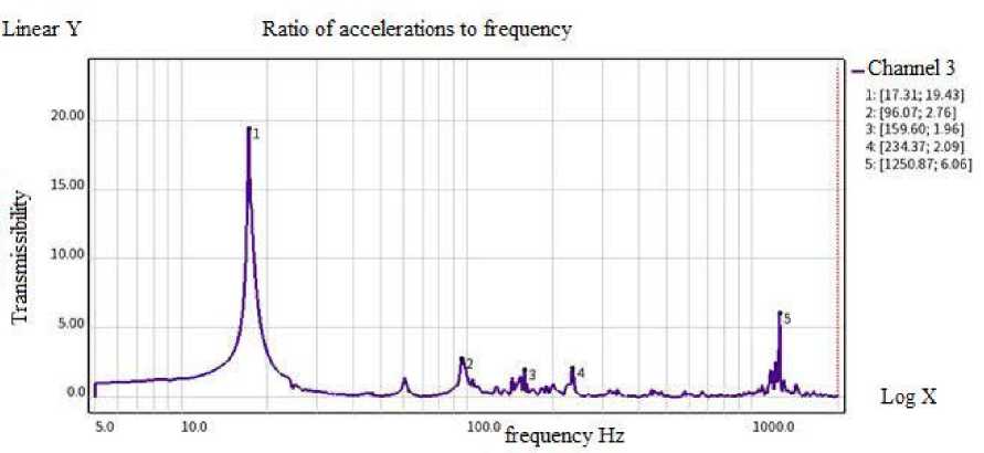
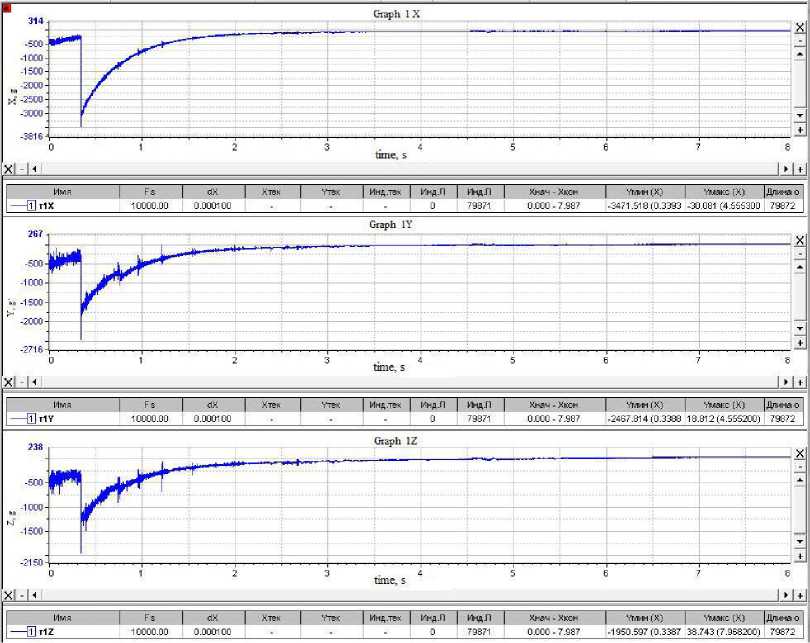
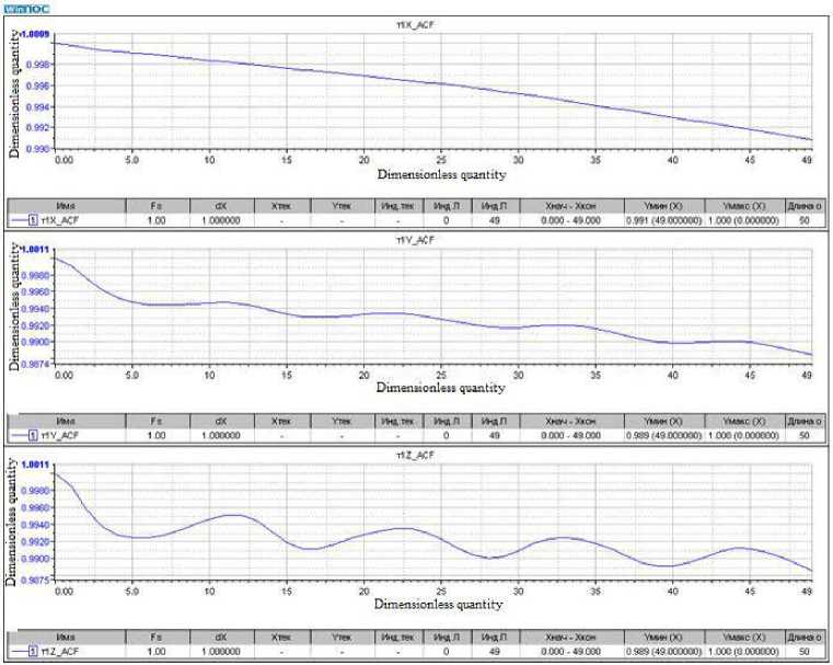
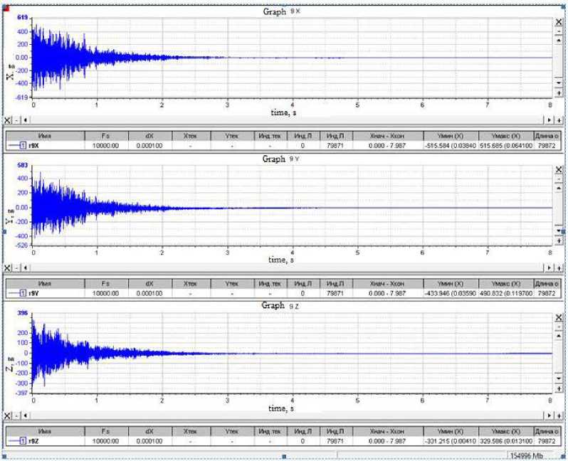
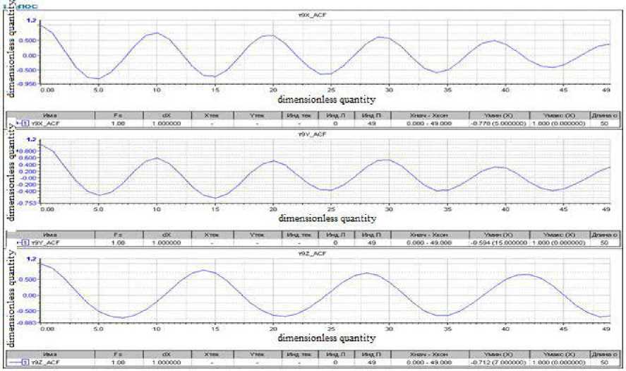
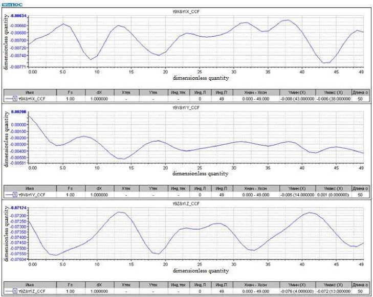
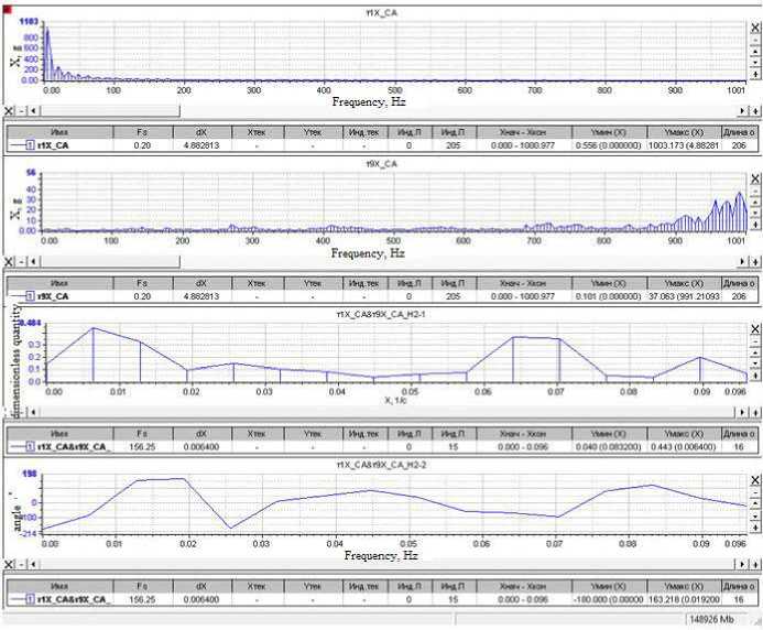
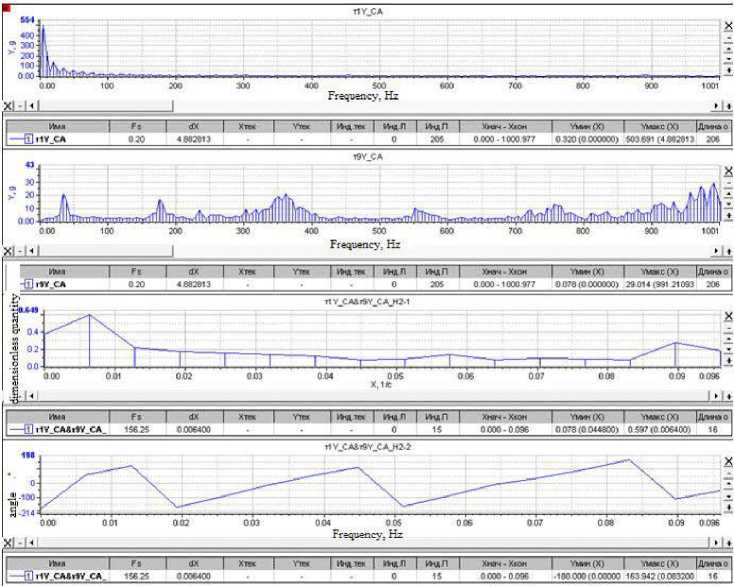
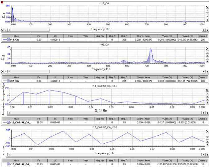
5 (f ) = 4jp(?) cos2nf т d т;0 < f where ρ(τ) is the normalized dimensionless correlation function; τ is the correlation time. Any signal that has periodic components can be decomposed into sinusoids of various frequencies, i.e. in a Fourier series. When processing vibrational accelerations represented by digital signals, a discrete Fourier transform F (n, N) is used to select a random process {xk, k = 0, ... N-1}, i.e. in a generalized form called AutoSpectrum, i n-1 _ j 2nkn F [n• N] = ^ Xke N . (15) N k=0 Based on the discrete Fourier transform F(n, N), the following types of spectral characteristics are determined: power spectrum, amplitude spectrum, power density spectrum, energy density spectrum [10–18]. Power Spectrum (PS). PS is a characteristic determined by averaging over M implementations and has the dimension (m/s2)2. It is determined by the dependence [12; 17–18] M M 2M GCM (n. T ) = ^ ZGCMj (n. T )= Й Z |Fj( n. N )| = ЙЙ Zl F;( n • N) •(16) where F (n •N )=ijn •N) •( Here T is the observation interval. The WinPos software package calculates a one-sided power spectrum and uses weight windows, so correction factors must be introduced: 2 Kн Gcm (n • T) GС M(n • T )= ККУМ • (18) where 2 indicates that we are calculating a one-sided power spectrum; Kн = 1 for effective values; Kн = 2 for peak values; KКУМ – coherent power gain (equal to the square of the coherent gain), depends on the choice of the weighting function. The amplitude spectrum is determined through the power spectrum and has the dimension - m/s2 Ga ( n, T) = ^GcM( n, T) . (19) Power Density Spectrum (PDS). The characteristic is defined as an average over M implementations and has the dimension - (m/s2)2/Hz: GcnM [ n T ] = г Gcm , (20) Af where ∆f is the polling frequency. Energy Density Spectrum (EDS). Averaging is performed over M implementations, the dimension of the characteristics of the operation of the EDS is (s (m/s2) 2 / Hz): Gens (n, T ) = ^ Ьспэ (n, T ) = ^ ^епм (n,T)’ T = GcnM (n, T \ T, (21) M j-0 M j=0 where T is the observation interval. For the oscillation period of the main vibration process component, it is possible to single out the effective (rms) value x (t); for complex vibration this value is chosen as the average between the effective and peak values. For vibration generated by harmonic vibrations f1, f2, f3, … с А1, А2, А3, … Акв=7 А+А2+Аз+... А2. When analyzing a stationary random process, the estimate of its theoretical spectral density is associated with averaging over an infinite ensemble. Therefore, a statistical estimation of the spectral density is usually performed, while the signal is passed through a narrow-band filter with a weight function h(t) tuned to a certain frequency ω0 [7–23]. The frequency components of the sample near ω0 are squared, by means of a quadrator device, and averaged. For processing normal random functions x(t) having spectral density with a pronounced sharp maximum, the envelope method is used, i.e. the original function is represented by two other functions of changing the amplitude A(t) and phase Ф(t), where A(t) obeys the Rayleigh distribution: X (t ) = A (t) cos Ф (t). (23) Then, assuming the linearity of the dependence of the phase Ф (t), for an approximate estimate of the correlation dependences of the amplitude and phase, simplifications are applied [7–8; 15–20]. Narrow-band vibrational processes are considered as a response of a dynamic system with low damping to broad-band disturbances, which are Gaussian white noise. In the case of an implementation with sharp peaks of resonances, the mathematical expectation of the frequency ω0 coincides with the natural frequencies values. One can assign the envelope A(t) of a narrow-band random process through the mathematical expectation of the frequency ω0 A (t ) = x2(t) + x3^. ®0 The one-dimensional probability density of the envelope A(t) obeys the Rayleigh distribution law ( Y- } jмакс P = ? exp Y2 ^ jмакс J here Yj макс are the values of peak overloads. The value of the standard deviation σ can be determined as the response of a structure to a broadband random vibration by summing up a number of narrowband actions a = n Em (.fj )afj j=1 where βfj is the dynamic-response factor (see formulas (3)–(4)) of the ratio of the base displacement amplitude to the driving force amplitude at a given frequency; S (fj) is the spectrum density of random vibration components in the frequency band ∆f; N is the number of partitioning intervals of the analyzed frequency band. The dynamic connection or conduction of vibrations by the structural elements of the rocket carriage between the sensors is determined by the transfer function. The transfer function in the frequency domain displays the ratio of output values to input values of various systems and characterizes stable, linear, time-invariant physical systems (mechanical, acoustic and electrical). Based on the results of simultaneous measurements and signal processing based on the fast Fourier transform (FFT) method and signals analysis at the input and output of the dynamic link, two different estimates of the complex frequency response of this system can be determined [12; 18], i.e. H1 (k) = SAB (k) / Saa (k) и H2 (k) = SBB (k) / SBA (k). (27) Here a(t) is the signal at the system input; b(t) is the signal at the output of the system. When the structure is exposed to vibrations with a variable frequency, the resonances of the system will be realized sequentially. Vibration resistance of the design depends on the density level of the spectrum, the bandwidth of the exciting frequencies, and the number of elements resonances that occur simultaneously. Such an impact can be critical from the point of vibration strength of the sled structural elements or the tested product itself [19–23]. Dynamic characteristics of rocket track sled 33AB-NO505 No. 2 There are the following types of mechanical tests: bench, full-scale on model modes and full-scale tests in operational conditions. Bench tests are carried out in order to determine natural resonances in a given frequency range; vibration strength tests; vibration resistance in a given frequency range; resistance to shock and vibro-impact loads. In this work, bench and full-scale tests in operational conditions were performed. To measure vibrations on the rocket sled, three-channel vibration acceleration sensors AP-2045-1, АР-2043-10 were installed, positioned along the X, Y, Z axes. The sensors were placed at various points on the surfaces of the structural elements of the sled and the model test object. The layout of sensors and registration drives is shown in fig. 2. Range of maximum values of measured accelerations by AP-2045-1 sensors is up to 5000 g and by АР-2043-10 sensors up to 500 g. The error of the sensors on average does not exceed 5%. The X axis of the sensors is set in the direction of movement. The Y-axis is perpendicular to the X-axis and is directed vertically upwards. The Z axis, in turn, is perpendicular to the X and Y axes. Along the Z axis, the sensors register lateral vibration accelerations. Рис. 2. Схема размещения датчиков вибраций и вторичных преобразователей-накопителей на каретке с размещенным модельным изделием Fig. 2. Scheme of placement of vibration sensors and secondary converters-drives on a sled with a placed model product To determine the frequency of natural resonances of some oscillation modes of the rocket sled and its dynamic characteristics, bench tests were carried out for scanning broadband sinusoidal disturbances in the vertical direction, including impact. Fig. 3 shows one of the fragments of the results of bench tests of the sled 33AB-NO505 No. 2. Рис. 3. Зависимость динамического коэффициента передачи (резонансного усиления) от частоты вынужденных колебаний Fig. 3. Dependence of the dynamic transmission coefficient (resonant amplification) on the frequency of forced oscillations As a result of bench tests of the dynamic response, measured by sensors located at various points in the design of the rocket track sled, being exposed to broadband sinusoidal disturbances, including impact, the amplitude-frequency characteristics of the sled were determined, and the resonant frequencies of its elements were identified (calculation of dynamic coefficients) in the frequency range 5-2000 Hz. Fig. 3 on the right shows the resonant frequencies and the values of the gains for channel 3. However, the rigid fastening of the sled structure with a section of the rail to the table of the shaker differs from the actual conditions when the carriage moves, therefore, the obtained resonant frequencies and the values of the dynamic coefficients for the sled elements are indicative. Signal Processing Algorithm for Vibration Acceleration Sensors and a Method for Determining the Dynamic Characteristics of Rocket Track Sled Elements We will present the sequence of processing and analysis of signals from vibration acceleration sensors using the example of one of the fire launches of a rocket track carriage with a test object in the form shown in Fig. 1. The purpose of this test cycle was to determine the maximum vibrations of the sled structural elements when it reaches the speed of 360 m/s2 which slightly exceeds the speed of sound. Figure 4 shows the recorded signals of vibrational accelerations along the X, Y and Z axes by sensor No. 1, located in the right front slipper of the rocket sled (see Fig. 2). To obtain reliable results, the original signal must be narrowband and centered. Filtering is used to eliminate noise when processing signals with a significant noise background. It is also possible to use the signal envelope to exclude noise (see formulas (23) - (26)). The algorithm for determining the envelope of signals in a discrete form is written as follows [18]: Yn'= Уn-1 +(1 xn| -Уn-1 ) / K , where K is the coefficient "RC" - averaging: K = RC/Δt, Δt - sampling time; f yn _ при_ yn ^ xn, у n = 1 Ixn_при_Уn ^ xn. The K factor determines the "time constant" of the peak detector. The prime in the parameter labels means the use of the weight window in signal processing. In this case, when calculating, it is necessary to introduce correction factors [18]. From fig. 4 it follows that the right front support of the sled was subjected to impact for 0.33 s. The maximum value of impact on the X axis is nx= -350 g, on the Yn axis = -250 g, and on the Z n axis = -190 g. At the previous moment of time, the largest disturbance was registered along the Z axis and was equal to n = -51 g. The probable cause of the impact could be the loss of support stability due to movable contact with the joint between the rails or due to the geometrical unevenness of the rail. The shock contact of the right support with the rail in the horizontal plane along the Z axis initiated a synchronous shock pulse in the direction of the Y and X axes. Table 1 shows the calculated values of the signals probabilistic characteristics: mathematical expectation; dispersion; standard deviation; asymmetry coefficient of distribution density; kurtosis for estimating the peaked distribution in relation to the normal distribution law; root mean square (RMS) -it is equal to the square root of the arithmetic mean of the squared deviations of the signal. Table 1 Probabilistic characteristics of sensor signals No 1 № М[X2] D[X] Ox Asymmetry Kurtosis Amplitude RMS 1X -246.096 213016 461.536 -3.51491 16.0719 1720.72 523.045 1Y -146.259 81580,5 285.623 -2.89054 12.0199 1243.31 320.891 1Z -110.66 49495.7 222.476 -2.62315 10.4763 994.67 248.477 Рис. 4. Сигналы виброускорений по осям X,Y, Z датчика № 1. По оси ординат значения ускорения приведены в g Fig. 4. Vibration acceleration signals along the X,Y, Z axes of sensor No. 1. Along the ordinate axis, acceleration values are given in g For a sequence of readings {xk, k = 0, ... N-1}, the estimates of the above characteristics are calculated using the following formulas [12–18]: 1 N-1 - expected value MI X2I = — У x,; N^ 1 N-I 2 - dispersion D [X] =----У (x; - m ) characterizes the dispersion of the values of a random N — 1 to' variable relative to its expected value; - standard deviation °x = ^Dx characterizes dispersion, but has the dimension of a random variable; 1 N-I 3 - assymenty Sk =---- У (x - m ) serves to evaluate the characteristics of the "skewness" of n< i=0 the distribution. If the distribution is symmetrical with respect to the expected value, then the skewness is 0; 1 N-1 4 - kurtosis E =---~У (x - mx) - 3 characterizes the peak or it has a flatter top of the N° 4 t0 distribution. For a normal distribution, the kurtosis is 0. Curves that are more pointed than the normal distribution have positive kurtosis. Flat-topped curves are characterized by negative kurtosis. Figure 5 shows graphs of autocorrelation functions of sensor signals No. 1. Рис. 5. Автокорреляционные функции (АКФ) сигналов по осям X, Y, Z датчика № 1 Fig. 5. Autocorrelation functions of signals along the XYZ axes of sensor No. 1 In a two-dimensional vector space, one parameter that measures a quantity is not enough, therefore, a pair of mutually perpendicular vectors, called an orthonormal basis, is used. A vector with a norm equal to one is called a unit vector (see formula (13)). Such a pair of vectors makes it possible to measure the required quantity. The correlation coefficient is a value that depends on the angle of the vector and does not depend on its modulus. It is possible to calculate the normalized correlation coefficient of various signals regardless of their physical properties and their magnitude. Autocorrelation is a function that characterizes the same signal considered at different time t and (t + τ). With autocorrelation, you can analyze a signal for the presence of a periodic component or periodic properties of the signal. The ACF is an even and decaying function if the random process does not contain a constant value. Autocorrelation functions vary from one to zero. The autocorrelation function of a periodic signal is always a periodic function. Masking noise (background noise) is usually a random signal, the amplitude of the autocorrelation function of which decreases with increasing time delay and, after a certain time, takes on a value equal to zero. Therefore, using the autocorrelation function, it is possible to detect a periodic signal after the time required for the disappearance of the noise component. Figure 5 shows the graphs of the ACF of the signals along the X, Y and Z axes, which are slightly different. The period of the harmonic component can be distinguished along the Y and Z axes. Along the X axis, the periodic component is not visually visible. Figure 6 shows the signals of vibration acceleration sensor No. 9, located on the surface of the fairing (see Fig. 2). Рис. 6. Сигналы виброускорений по осям X, Y и Z датчика № 9. Размерность оси ординат в g Fig. 6. Vibration acceleration signals along the X, Y and Z axes of sensor No. 9. The dimension of the ordinate axis is in g Table 2 Probabilistic characteristics of sensor signals No. 9 № М[X2] D[X] σx Asymmetry Kurtosis Amplitude RMS 9X –1.18734 2059.6 45.3828 –0.100333 28.135 515.634 45.398 9Y –5.4057 1392.65 37.3182 0.452846 25.4988 462.389 37.7075 9Z –3.8819 724.405 26.9148 0.567577 28.4485 330.4 27.1931 The signals registered by sensor No. 9, in contrast to the shock pulses of sensor No. 1, are periodic in nature and include an impulse disturbance for 0.33 s. Figure 7 shows the signal envelopes along the X, Y, Z axes of sensor No. 9. Fig. 7 shows the autocorrelation functions of the signals from sensor No. 9. The ACFs of all sensors No. 9 signals illustrate harmonic signals with very slowly varying amplitude and phase. A change in the amplitude of the ACF characterizes the smallness of the vibrational energy loss or the small value of the oscillation damping coefficient. We can see the phase shift of the ACF signal along the Z axis relative to the ACF of the signals along the X and Y axes, and we can also distinguish a different period for all three signals. The amplitude of the normalized autocorrelation function of a broadband random signal (noise) should rapidly decrease to zero in accordance with the so-called law of uncertainty of functions coupled via the Fourier transform [20– 23]. This law relates the bandwidth ∆f of the intrinsic spectrum Gaa (f) and the duration ∆t of the corresponding autocorrelation function Raa(t) in the form Δf·Δt ≥ 1. In order to detect a periodic signal containing several frequency components, it is often more appropriate to use autocorrelation function, but its own spectrum. Based on the intrinsic spectrum, it is possible to determine both the frequencies and the amplitudes of the individual components of the noise-masked periodic signal. However, if the amplitudes of these components are small compared to the level of the masking signal (background noise), then it is necessary to carry out the analysis with frequency upscaling. Fig. 8 shows the cross-correlation function between the corresponding signals of sensors No. 9 and 1. Рис. 7. АКФ сигналов X, Y, Z датчика виброускорений № 9 Fig. 7. Autocorrelation functions of signals X, Y, Z of vibration acceleration sensor No. 9 The cross-correlation function is used to determine the similarity or difference between two periodic signals. The cross-correlation coefficient varies from –1 to +1; the maximum of the function can be shifted relative to the middle. Using the cross-correlation function, you can determine the strength of the connection between two signals, as well as the degree of delay. This function is symmetrical, at τ = 0 it takes on a maximum value and the peaks at the points of this function give a period nt. According to the graphs above, in a certain frequency range (from 10 to 27 units), one can see the similarity of signals along the Z and X axes, which indicates the mutual connection of vibration processes along the Z and X axes in point 9. Figures 9–11 show graphs of the densities of the amplitude spectra (SA) along the X, Y, and Z axes of sensors No. 1 and 9, as well as graphs of the signal gains of the transfer functions along the X, Y, and Z axes, determined from the densities of the SA spectra. The upper graphs represent the density distributions of the amplitude spectra over frequency in the range from 0 to 1000 Hz. The middle graph shows the numerical values of the dynamic coefficients (amplification or attenuation) of signals distributed over the same frequency range from 0 to 1000 Hz. The dimension of the X-axis is 1/s (1/Hz). The graph below depicts the corresponding phase shifts between the signals. In the low frequency range, the dynamic coefficient of signals along the X axis between sensors No. 1 and 9 is less than one, i.e., the vibration is transmitted with attenuation. Figure 10 shows the density of the spectra and the dependence of the transmission coefficient for signals along the Y axis. Рис. 8. Взаимная корреляционная функция сигналов по осям X, Y, Z между датчиками № 9 и 1 Fig. 8. Mutual correlation function of signals along the X, Y, Z axes between sensors No. 9 and 1 Рис. 9. Графики плотности спектров амплитуды сигналов по оси Х датчиков № 1 и 9. Зависимости динамических коэффициентов передаточной функции Н2 (f) по оси X сигналов датчиков № 1 и 9. Сдвиг фазы между соответствующими сигналами в зависимости от частоты Fig. 9. Graphs of the spectral density of the signal amplitude along the X axis of sensors No. 1 and 9. Dependences of the dynamic coefficients of the transfer function H2 (f) along the X axis of the signals of sensors No. 1 and 9. Phase shift between the corresponding signals depending on the frequency Рис. 10. Графики плотности спектров амплитуды сигналов по оси Y датчиков № 1 и 9. Зависимости динамических коэффициентов передаточной функции Н2 (f) по оси Y сигналов датчиков № 1 и 9. Сдвиг фазы между соответствующими сигналами в зависимости от частоты Fig. 10. Graphs of the spectral density of the signal amplitude along the Y axis of sensors No. 1 and 9. Dependences of the dynamic coefficients of the transfer function H2 (f) along the Y axis of the signals of sensors No. 1 and 9. Phase shift between the corresponding signals depending on the frequency Vibration along the Y axis is directed vertically upwards. In the frequency range from 0 to 1000 Hz, in general, the dynamic coefficient of the signals of sensors No. 1 and 9 along the Y axis is less than one. However, at frequencies around 70 Hz, the dynamic coefficient is maximum. In the frequency range from 0 to 650 Hz, the dynamic coefficient of the signals of sensors No. 1 and 9 along the Z axis is significantly greater than unity. Resonant amplification of the signal is noted, at a frequency of 70 Hz the coefficient is K = 5.6, then at 190 Hz K = 6.4. At a frequency of 600 Hz, the transmission coefficient decreases, but its value is still greater than unity K = 2.3. Further, as the frequency increases from 650 to 1000 Hz, it becomes close to unity. From this we can conclude that the lateral vibration in the horizontal plane along the Z axis is transmitted from the slippers of the rocket sled to the nose fairing with amplification in the low-frequency range from 15 to 400 Hz. The vibration of the slippers in the vertical direction along the Y axis, which occurs when they slide along the surface of the rail guides, is transmitted to the fairing in a significantly weakened form. This is due to the mass of the movable track sled effects. Based on the obtained results of signal processing, it can be concluded that the conductivity of vibrations arising from the dynamic interaction of the front sliding bearing along the contact surface of the rail track to the test object is realized with attenuation. However, near some natural resonances of the rocket sled in the frequency range from 15 to 600 Hz, an increase in the dynamic coefficient along the Z axis to a value of 8.0 is observed. Vibrations in the transverse plane along the Z axis are the source of bending and torsional vibrations of structural elements, which are most critical in high-speed testing of products, since the stability of the movement of the rocket sled and the vibration strength of the slippers depend on these vibrations. Рис. 11. Графики плотности спектров амплитуды сигналов по оси Z датчиков № 1 и 9. Зависимости динамических коэффициентов передаточной функции Н2 (f) по оси Z сигналов датчиков № 1 и 9. Сдвиг фазы между соответствующими сигналами в зависимости от частоты Fig. 11 Graphs of the spectral density of the signal amplitude along the Z axis of sensors No. 1 and 9. Dependences of the dynamic coefficients of the transfer function H2 (f) along the Z axis of the signals of sensors No. 1 and 9. Phase shift between the corresponding signals depending on the frequency Conclusion High-speed ground track tests of aviation and rocket products are accompanied by intense vibration of the rocket sled elements and the test object. The developed methodological sequence of statistical processing of the results of recording vibration acceleration sensors located at various points in the rocket sled structure makes it possible to determine the distributions of the power spectrum density and energy spectrum density over frequency; estimate autocorrelation dependencies, probability densities of stochastic vibration signals and also calculate the mutual correlation functions and transfer functions of the compared signals at various points of the structure in order to determine the conductance dynamic coefficients of harmonic and shock disturbances by the elements of the structure. The example of processing vibration accelerations given in the article is the basis for systematic studies of the dynamic characteristics of random signals with the naim to develop means for damping vibrations in the process of product ground track testing at a speed exceeding 3M.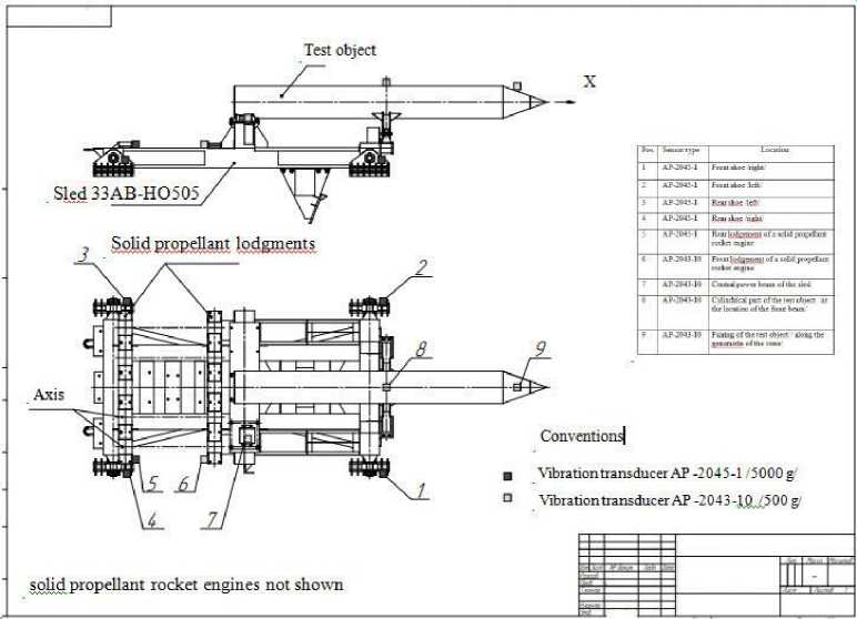
References Experimental determination of vibration conductivity by rocket sled structural elements in high-speed track tests of aircraft equipment
- Timoshenko S. P., Yang D. K., Uiver U. Kolebaniya v inzhenernom dele [Fluctuations in engineering]. Moscow, Mashinostroenie Publ., 1985, 472 p.
- Gorshkov A. G., Medvedskii A. L., Rabinskii L. N., Tarlakovskii D. V. Volny v sploshnykh sredakh [Waves in continuous media]. Moscow, Fizmatlit Publ., 2004, 472 p.
- Astakhov S. A., Biryukov V. I., Kulak I. P., Chernykh A. S., Khamzatkhanov S. A. [Bending-torsional oscillations of a cantilevered streamlined body with an annular cross section during high-speed track tests]. Materialy XXVIII Mezhdunarodnogo simpoziuma «Dinamicheskie i tekhnologicheskie problemy mekhaniki konstruktsii i sploshnykh sreD» im. A.G. Gorshkova. 2022, Vol. 2, P. 12–14.
- Erofeev V. I., Kazhaev V. V., Semerikova N. P. Volny v sterzhnyakh. Dispersiya. Dissipatsiya. Nelineinost' [Waves in Rods. Dispersion. Dissipation. Nonlinearity]. Moscow, Fizmatlit Publ., 2002, 208 p.
- Vibratsii v tekhnike [Vibrations in technology]. Ed. Bolotina V. V. 1999, 504 p.
- Artobolevskii I. I., Bobrovnitskii Yu. I., Genkin M. D. Vvedenie v akusticheskuyu dinamiku mashin [Introduction to the acoustic dynamics of machines]. Moscow, Gl. red. fiz.-mat. lit. Publ, 1979, 296 p.
- Iorish Yu. I. Vibrometriya [Vibrometry]. Moscow, Mashgiz Publ., 1963,773 p.
- Karpushin V. B. Vibratsii i udary v radioapparature [Vibrations and shocks in radio equipment]. Moscow, Sov. Radio Publ., 1971, 344 p.
- Anan'ev I. V., Timofeev P. G. Kolebaniya uprugikh sistem v aviatsionnykh konstruktsiyakh i ikh dempfirovanie [Oscillations of elastic systems in aviation structures and their damping]. Moscow, Mashinostroenie Publ., 1965, 526 p.
- Dmitriev B. M. Otsenka dopustimykh mekhanicheskikh nagruzok dlya izdelii [Evaluation of allowable mechanical loads for products]. Moscow, Mashgiz Publ., 1973, 39 p.
- Astakhov S. A., Biryukov V. I. Problems of ensuring the acceleration dynamics of aircraft during track test at a speed of 1600 m/s. INCAS BULLETIN. 2020, Vol. 12, P. 33–42. DOI: 10.13111 / 2066-8201.2020.12.S.3; https://doi.org/10.13111/2066-8201.2020.12.S.3.
- Mirskii G. Y. Apparaturnoe opredelenie kharakteristik sluchainykh protsessov. Izdanie 2-e pererabotannoe i dopolnennoe [Apparatus determination of the characteristics of random processes]. Moscow, Energiya Publ., 1972, 456 p.
- Pugachev V. S. Teoriya sluchainykh funktsii i ee primenenie k zadacham avtomaticheskogo upravleniya [Theory of random functions and its application to automatic control problems]. Moscow, Fizmatgiz Publ., 1960, 883 p.
- Kharkevich A. A. Spektry i analiz [Spectra and Analysis]. Moscow, Fizmatgiz Publ., 1962, 236 p.
- Bendat Dzh., Pirsol A. Primeneniya korrelyatsionnogo i spektral'nogo analiza [Applications of correlation and spectral analysis: translation from English]. Moscow, Mir Publ., 1983, 312 p.
- Shkalikov V. S., Pellinets V. S., Isakovich E. G. et al. Izmerenie parametrov vibratsii i udara [Measurement of vibration and shock parameters]. Moscow, Standartizdat Publ., 1980, 280 p.
- Stiven Smit Tsifrovaya obrabotka signalov. Prakticheskoe rukovodstvo dlya inzhenerov i nauchnykh rabotnikov [Stephen Smith. Digital signal processing. A practical guide for engineers and scientists]. Moscow, Dodehka-KHKH1 Publ., 2012, 720 p.
- Paket prikladnykh programm WIN POS MERA [Package of applied programs WIN POS MERA]. Avaitable at: www.nppmera.ru.
- Sergeev S. I. Dempfirovanie mekhanicheskikh kolebanii [Damping of mechanical vibrations]. Moscow, Fizmatgiz Publ., 1959, 408 p.
- Yavlenskii A. K., Yavlenskii K. N. Vibrodiagnostika i prognozirovanie kachestva mekhanicheskikh system [Vibrodiagnostics and prediction of the quality of mechanical systems]. Leningrad, Mashinostroenie Publ., 1983, 239 p.
- Bobrovnitskii Y. I., Genkin M. D., Morozov K. D. [New method of acoustic diagnostics]. Dinamika i akustika mashin. Moscow, Nauka Publ., 1971, P. 98–108.
- Genkin M. D., Sokolova A. G. Vibroakusticheskaya diagnostika mashin i mekhanizmov [Vibroacoustic diagnostics of machines and mechanisms]. Moscow, Mashinostroenie Publ., 1987, 288 p.
- Vibratsiya ehnergeticheskikh mashin: sprav, posobie [Vibration of power machines: Ref. allowance]. Ed. N. V. Grigorieva. Leningrad, Mashinostroenie Publ., 1974, 464 p.
