Experimental study of the effect of the roughness of additively fabricated surfaces on the hydrodynamics of cooling paths of liquid rocket engines

Author: Manokhina E.S., Ivanov A.S., Zuev A.A., Arngold A.A.
Journal: Siberian Aerospace Journal @vestnik-sibsau-en
Section: Aviation and spacecraft engineering
Article in issue: 1 vol.27, 2026.
Free access
Increasing the efficiency of liquid rocket engines (LRE) is inextricably linked to the intensification of cooling processes in heat-critical elements such as combustion chambers and nozzles. Additive Manufacturing (AM) technologies, in particular selective laser fusion (SLM), make it possible to create cooling paths with complex internal channels and heat transfer intensifiers. However, the surface microrelief formed in this case has a significant effect on hydrodynamic resistance and heat transfer, which is not always taken into account in existing design methods. An experimental assessment of the effect of surface roughness, characteristic of additive manufacturing, on the formation of a dynamic boundary layer under conditions simulating flows in the cooling channels of liquid propellant is considered. The sample plates made of AlSi10Mg aluminum alloy were made using the SLM method: with controlled roughness and flow intensifiers. The surface roughness profile was evaluated on a TR 110 profilometer. The research was carried out on a specially designed aerodynamic installation that simulates the flow in a rectangular channel. The velocity fields in the wall area were measured by the pneumometric method at a fixed air flow rate. The errors were estimated and the data approximated. It is established that the roughness of SLM surfaces leads to a significant restructuring of the velocity profile in the boundary layer compared to the hydraulically smooth case: a decrease in its thickness and a change in the shape of the velocity diagram are observed. The largest deviations were recorded for the plate with intensifiers. Power-law approximating dependences are obtained for each type of surface, where the exponent varies depending on the roughness parameters. It is shown that the use of boundary layer models for smooth surfaces in liquid propellant calculations in relation to additive parts can lead to incorrect estimation of hydraulic losses and, as a result, to errors in predicting the temperature state of the wall. The obtained dependences are necessary for the development of adjusted calculation methods that take into account the actual topography of the surfaces formed by AM methods, which will increase the reliability and efficiency of the design of liquid propellant cooling systems.
Liquid rocket engine, cooling path, additive manufacturing, selective laser fusion, boundary layer, surface roughness, hydrodynamic resistance, heat transfer
Short address: https://sciup.org/148333274
IDR: 148333274 | UDC: 621.45 | DOI: 10.31772/2712-8970-2026-27-1-123-140
Text of the scientific article Experimental study of the effect of the roughness of additively fabricated surfaces on the hydrodynamics of cooling paths of liquid rocket engines
Improving the energy-mass efficiency of liquid rocket engines (LREs) is one of the key challenges in modern rocketry. The solution to this challenge is largely determined by the capabilities of cooling systems for critical components, such as the combustion chamber and nozzle, operating under extreme heat fluxes. Traditional manufacturing methods for these components impose significant limitations on the geometry of the internal surfaces of the cooling ducts.
Additive manufacturing (AM), particularly selective laser melting (SLM), opens up new possibilities, enabling the creation of complex cooling systems with complex channel networks, turbulators, and other heat transfer enhancers integrated directly into the wall structure. However, the layer-bylayer synthesis process results in the formation of a specific surface microrelief, which can dramatically affect processes in the near-wall region of coolant flow.
As is well known, in a viscous fluid, the no-slip condition is realized near the wall, and the transition from zero velocity at the wall to the external flow velocity occurs in a thin region – the dynamic boundary layer [1; 2]. Similarly, the temperature change between the wall and the flow occurs in the thermal boundary layer [3–9]. These two layers are closely related, and their relative thickness is determined by the dimensionless Prandtl number (Pr).
In liquid propellant rocket engine components, the flow in the cooling channels is turbulent and characterized by high Reynolds numbers [10–16]. Heat transfer processes and hydrodynamic losses under such conditions are determined by the structure of the dynamic and thermal boundary layers. For gases, the Prandtl number is close to unity, which means that the thicknesses of the dynamic and thermal boundary layers are commensurate [3]. Consequently, determining the characteristics of the dynamic layer allows one to indirectly assess heat transfer processes [17–22].
Existing semi-empirical models and correlations for friction and heat transfer used in design were developed for standard (hydraulic smooth) surfaces. Their application to additively manufactured parts without taking into account the actual roughness can lead to significant errors in calculating the pressure drop and wall temperature field, which is unacceptable when designing highly loaded liquid-propellant rocket engine components.
The concept of sand roughness and the associated classical formulas are inapplicable to surfaces produced by SLM, as this model assumes a uniform and isotropic distribution of identical protrusions described by a single parameter—the height k_s. In reality, an SLM surface has a complex, nonuniform, and anisotropic microrelief (droplets, overhangs, welded particles), whose statistical parameters (Ra, Rz) vary greatly, and its hydrodynamic influence cannot be reduced to an equivalent sand grain height. Moreover, SLM parts often contain macroscopic elements (intensifiers) that fundamentally go beyond the sand roughness model, requiring the development of new experimental relationships. This is confirmed by a study demonstrating different patterns of velocity profile changes for different types of additively machined surfaces.
Thus, the aim of this work is to experimentally study the formation of a dynamic boundary layer on surfaces simulating the internal cooling channels of a liquid-propellant rocket engine, manufactured using the SLM method, with a quantitative assessment of the influence of roughness and macroscopic inhomogeneities on the velocity profile. To achieve this goal, an experimental setup was developed, velocity field measurements were carried out, an error assessment was performed, and an approximation of the obtained data was carried out for subsequent use in hydrodynamic and thermal calculations [1–3].
Description of the experimental setup and bench
The experimental setup (Figs. 1, 2) and the installation are designed to simulate coolant flow (in this case, air) in a rectangular channel, hydrodynamically similar to the cooling ducts of liquidpropellant rocket engines. The inlet section, 10 hydraulic diameters long, ensures the formation of a stabilized turbulent flow ahead of the measurement zone, which corresponds to conditions in real engines.
The studies were conducted on a specially designed rig, the main components of which included a compressed air supply system (two sequential compression stages), an ASAIRAMS 1000 gas flow meter, a battery of seven HT-1890 differential pressure gauges (accuracy ±0.3%), and the experimental setup itself.
The experimental setup (Figs. 3–4) is a rectangular duct made of acrylic plexiglass, measuring 36×52 mm in cross-section and 372 mm in length. The duct housing contains seven static pressure sensors and seven total pressure sensors (2 mm diameter needles with a 1.2 mm orifice), spaced 50 mm apart along the duct axis. The static pressure sensors are installed in specially selected control sections of the flow path, where the flow is steady and there are no significant pressure gradients. They are mounted through pre-drilled holes in the duct walls, which are sealed to prevent leaks. The sensor axes are strictly perpendicular to the flow direction to minimize the influence of dynamic pressure. The total pressure sensors are bent at a 90° angle to align with the flow. A deflector and adapter, manufactured using FFF technology, are installed to equalize and stabilize the flow.
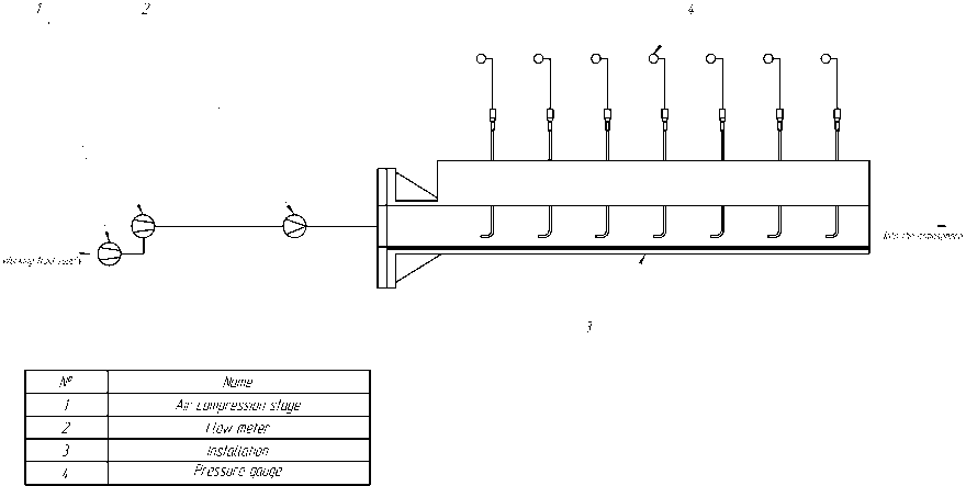
Рис. 1 Принципиальная схема стенда:
1 – ступень сжатия воздуха; 2 – расходомер; 3 – экспериментальная установка; 4 – манометр
Fig. 1 Schematic diagram of the setup:
1 – air compression stage; 2 – flow meter; 3 – pilot plant; 4 – pressure gauge
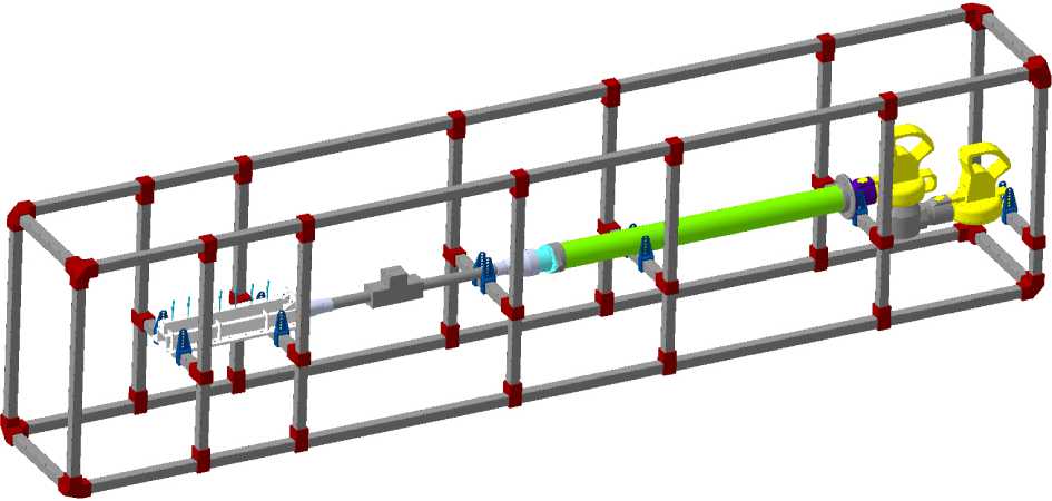
Рис. 2. 3Д-модель экспериментального стенда
-
Fig. 2. 3D model of the experimental stand
The key objects of the study (Fig. 5–7) were replaceable plates installed in the canal:
-
1. Hydraulically smooth plate (necessary for comparative analysis of the obtained experimental and theoretical data).
-
2. Roughened plates manufactured on a SLMASTRA 420 machine from ALSi10Mg alloy. The manufacturing process involved artificially creating different roughness on the front (side 1) and back (side 2).
-
3. Plate with flow intensifiers, also manufactured using the SLM method.
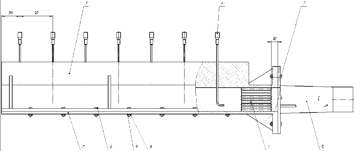
Рис. 3. Фрагмент сборочного чертежа установки
-
Fig. 3. Fragment of the assembly drawing of the installation
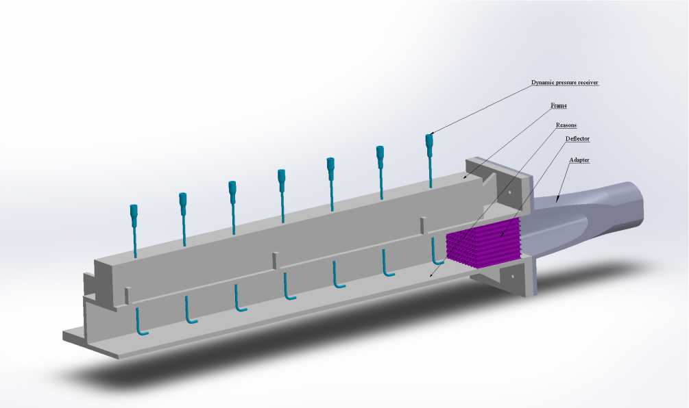
Рис. 4. 3Д-модель экспериментальной установки
-
Fig. 4. 3D model of the experimental setup
Surface roughness testing of the plates was performed using a TR 110 profilometer. Measurements of the Ra and Rz parameters were taken in the transverse direction at 30.4 mm intervals along the entire length of the plate. The measurement results are presented in Table 1 and Figs. 8–13, and the average values are presented in Table 2.
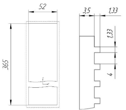
Рис. 5. Геометрические параметры пластин
Fig. 5. Geometric parameters of the plates
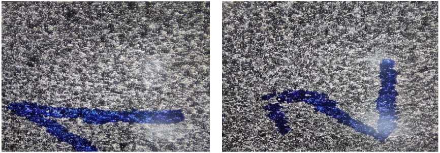
Рис. 6. 1 и 2 сторона шероховатой пластины при 50-кратном увеличении
Fig. 6. 1st and 2nd sides of a rough plate at 50x magnification
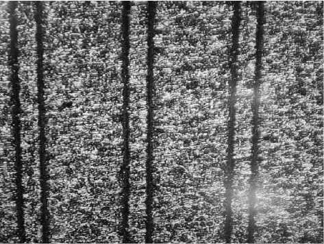
Рис. 7. Шероховатая пластина с интенсификаторами при 50-кратном увеличении
Fig. 7. Rough plate with intensifiers at 50x magnification
Table 1
|
Rough plate, 1 side |
Rough plate, side 2 |
Plate with intensifiers |
||||
|
L , mm |
Ra |
Rz |
Ra |
Rz |
Ra |
Rz |
|
30.42 |
1.67 |
5.92 |
5.91 |
28.2 |
9.43 |
42.1 |
|
60.83 |
0.19 |
1.47 |
7.93 |
24.7 |
0.66 |
3,27 |
|
91.25 |
5.89 |
18.96 |
3.5 |
17.72 |
4.59 |
23.2 |
|
121.66 |
1.39 |
8.21 |
2.56 |
9.46 |
6.46 |
27.8 |
|
152.08 |
2.16 |
10.3 |
7.89 |
25 |
1.58 |
8.69 |
|
182.5 |
2.75 |
7.48 |
7.68 |
23.6 |
3.68 |
16.17 |
|
212.91 |
2.17 |
8.15 |
4.21 |
17.76 |
7.1 |
30.3 |
|
243.33 |
4.61 |
12.53 |
4.06 |
15.18 |
4.21 |
15.69 |
|
273.75 |
1.14 |
6.45 |
5.11 |
19.11 |
0.95 |
4.2 |
|
304.16 |
3.21 |
15.52 |
6.22 |
21.6 |
3.59 |
7.44 |
|
334.58 |
1.48 |
7.91 |
4.05 |
15.35 |
0.19 |
0.99 |
|
365 |
0.97 |
3.9 |
4.85 |
21.9 |
2.95 |
14.26 |
Table 2
|
Rough plate, 1 side |
Rough plate, side 2 |
Rough plate with intensifiers |
|||
|
Ra |
Rz |
Ra |
Rz |
Ra |
Rz |
|
7.58 |
23.59 |
4.22 |
15.17 |
3.78 |
16.18 |
Results of roughness measurements on plates
Average roughness values
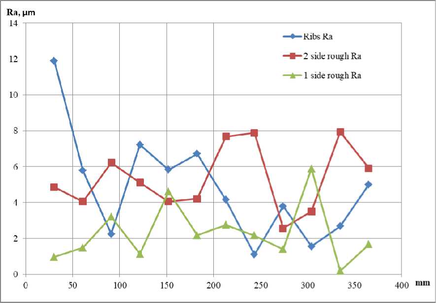
Рис. 8. Шероховатость по длине пластины, измеряемая по Ra
Fig. 8. Roughness along the length of the plate measured by Ra
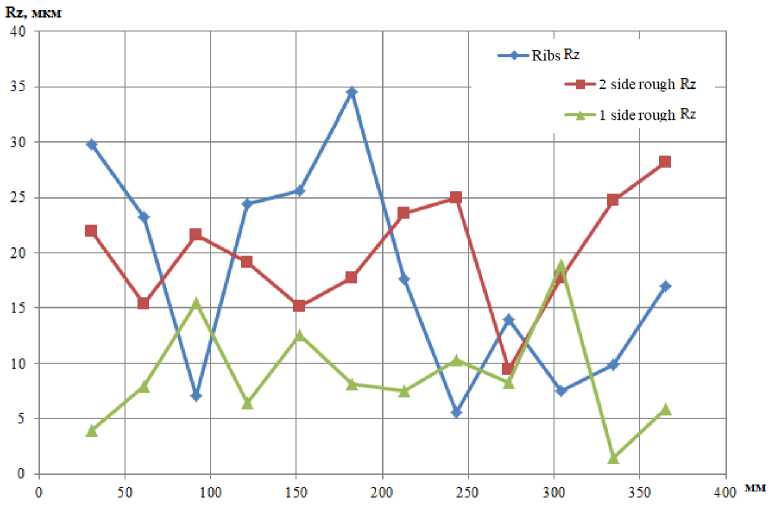
Рис. 9. Шероховатость по длине пластины измеряемая по Rz
Fig. 9. Roughness along the length of the plate measured by Rz
Methodology for processing experimental data
The flow velocity at various points in the boundary layer was determined using an indirect pneumometric method by measuring the static (Pst) and total (Pt) pressures. The volumetric air flow rate was monitored directly using a flow meter. Measurements were conducted at a flow rate of 1500 l/min. Air density was assumed constant (ρ = 1.127 kg/m³) for a room temperature of 25°C.
The local flow velocity (u) was calculated using the relationship:
u =

p d is the dynamic pressure at the measured point.
Research results
As a result of the experiments, velocity profiles were obtained for all types of surfaces. As a representative example, the article presents data for measurement section No. 6. The results are presented in dimensionless coordinates u/U (the ratio of the local velocity to the velocity at the outer boundary of the layer) and y/δ (the ratio of the distance from the wall to the boundary layer thickness δ). The experimental data are summarized in Tables 3–7 (Figs. 14, 15).
Table 3
Hydraulically smooth plate
|
№ |
y , mm |
P st, kPa |
P t , kPa |
u , m/s |
ρ, kg/m3 |
U , m/s |
u / U |
y /δ |
δ, mm |
U m |
|
1 |
0 |
60 |
60 |
0 |
1.127 |
34.22 |
0 |
0 |
13 |
27.97 |
|
2 |
0.5 |
60 |
270 |
21.88 |
0.63 |
0.03 |
||||
|
3 |
1 |
60 |
350 |
24.92 |
0.72 |
0.07 |
||||
|
4 |
2 |
60 |
380 |
25.96 |
0.75 |
0.15 |
||||
|
5 |
3 |
60 |
410 |
26.97 |
0.78 |
0.23 |
||||
|
6 |
4 |
60 |
440 |
27.94 |
0.81 |
0.3 |
End of table 3
|
№ |
y , mm |
P st, kPa |
P t , kPa |
u , m/s |
ρ, kg/m3 |
U , m/s |
u / U |
y /δ |
δ, mm |
U m |
|
7 |
5 |
60 |
480 |
29.18 |
0.85 |
0.38 |
||||
|
8 |
6 |
60 |
510 |
30.08 |
0.87 |
0.46 |
||||
|
9 |
7 |
60 |
550 |
31.24 |
0.91 |
0.53 |
||||
|
10 |
8 |
60 |
590 |
32.35 |
0.94 |
0.61 |
||||
|
11 |
9 |
60 |
620 |
33.17 |
0.96 |
0.69 |
||||
|
12 |
10 |
60 |
640 |
33.7 |
0.98 |
0.76 |
||||
|
13 |
11 |
60 |
650 |
33.96 |
0.99 |
0.84 |
||||
|
14 |
12 |
60 |
650 |
33.96 |
0.99 |
0.92 |
||||
|
15 |
13 |
60 |
660 |
34.22 |
1 |
1 |
Table 4
|
№ |
y , mm |
p Pst , kPa |
P t , kPa |
u , m/s |
ρ, kg/m3 |
U , m/s |
u / U |
y /δ |
δ, mm |
U m |
|
1 |
0 |
70 |
70 |
0 |
1.127 |
36.72 |
0 |
0 |
6 |
31.44 |
|
2 |
0.5 |
70 |
450 |
28.25 |
0.76 |
0.08 |
||||
|
3 |
1 |
70 |
570 |
31.8 |
0.86 |
0.16 |
||||
|
4 |
2 |
70 |
640 |
33.7 |
0.91 |
0.33 |
||||
|
5 |
3 |
70 |
670 |
34.48 |
0.93 |
0.5 |
||||
|
6 |
4 |
70 |
700 |
35.24 |
0.95 |
0.66 |
||||
|
7 |
5 |
70 |
730 |
35.99 |
0.98 |
0.83 |
||||
|
8 |
6 |
70 |
760 |
36.72 |
1 |
1 |
||||
|
9 |
7 |
70 |
760 |
36.72 |
||||||
|
10 |
8 |
70 |
760 |
36.72 |
Table 5
|
№ |
y , mm |
P st, kPa |
P t , kPa |
u , m/s |
ρ, kg/m3 |
U , m/s |
u / U |
y /δ |
δ, мм |
U m |
|
1 |
0 |
60 |
0 |
0 |
1.127 |
36.72 |
0 |
0 |
9 |
32.1 |
|
2 |
0.5 |
60 |
400 |
26.64 |
0.72 |
0.05 |
||||
|
3 |
1 |
60 |
500 |
29.78 |
0.81 |
0.11 |
||||
|
4 |
2 |
60 |
555 |
31.38 |
0.85 |
0.22 |
||||
|
5 |
3 |
60 |
600 |
32.63 |
0.88 |
0.33 |
||||
|
6 |
4 |
60 |
645 |
33.83 |
0.92 |
0.44 |
||||
|
7 |
5 |
60 |
680 |
34.73 |
0.94 |
0.55 |
||||
|
8 |
6 |
60 |
720 |
35.74 |
0.97 |
0.66 |
||||
|
9 |
7 |
60 |
735 |
36.11 |
0.98 |
0.77 |
||||
|
10 |
8 |
60 |
750 |
36.48 |
0.99 |
0.88 |
||||
|
11 |
9 |
60 |
760 |
36.72 |
1 |
1 |
Table 6
|
№ |
y , mm |
P st, kPa |
P t , kPa |
u , m/s |
ρ, kg/m3 |
U , m/s |
u / U |
y /δ |
δ, mm |
U m |
|
1 |
0 |
60 |
60 |
0 |
1.127 |
36.96 |
0 |
0 |
13 |
27.7 |
|
2 |
0.5 |
60 |
316.23 |
21.32 |
0.62 |
0.03 |
||||
|
3 |
1 |
60 |
372.35 |
23.54 |
0.69 |
0.07 |
||||
|
4 |
2 |
60 |
440.76 |
25.99 |
0.76 |
0.15 |
||||
|
5 |
3 |
60 |
487.52 |
27.54 |
0.81 |
0.23 |
||||
|
6 |
4 |
60 |
524.15 |
28.7 |
0.84 |
0.3 |
End of table 6
|
№ |
y , mm |
P st, kPa |
P п , kPa |
u , m/s |
ρ, kg/m3 |
U , m/s |
u / U |
y /δ |
δ, mm |
U m |
|
7 |
5 |
60 |
554.7 |
29.62 |
0.87 |
0.38 |
||||
|
8 |
6 |
60 |
581.16 |
30.41 |
0.89 |
0.46 |
||||
|
9 |
7 |
60 |
604.62 |
31.08 |
0.91 |
0.53 |
||||
|
10 |
8 |
60 |
625.8 |
31.68 |
0.93 |
0.61 |
||||
|
11 |
9 |
60 |
645.17 |
32.22 |
0.94 |
0.69 |
||||
|
12 |
10 |
60 |
663.05 |
32.71 |
0.96 |
0.76 |
||||
|
13 |
11 |
60 |
679.7 |
33.16 |
0.97 |
0.84 |
||||
|
14 |
12 |
60 |
695.3 |
33.57 |
0.98 |
0.92 |
||||
|
15 |
13 |
60 |
710 |
33.96 |
1 |
1 |
Table 7
|
№ |
y , mm |
P st, kPa |
P t , kPa |
u , m/s м/с |
ρ, kg/m3 |
U , m/s |
u / U |
y /δ |
δ, mm |
U m |
|
1 |
0 |
90 |
90 |
0 |
1.127 |
36.29 |
0 |
0 |
9 |
30.76 |
|
2 |
0.5 |
90 |
240 |
19.39 |
0.53 |
0.05 |
||||
|
3 |
1 |
90 |
370 |
24.08 |
0.66 |
0.11 |
||||
|
4 |
2 |
90 |
450 |
26.56 |
0.73 |
0.22 |
||||
|
5 |
3 |
90 |
530 |
28.82 |
0.79 |
0.33 |
||||
|
6 |
4 |
90 |
610 |
30.92 |
0.85 |
0.44 |
||||
|
7 |
5 |
90 |
690 |
32.89 |
0.9 |
0.55 |
||||
|
8 |
6 |
90 |
770 |
34.74 |
0.95 |
0.66 |
||||
|
9 |
7 |
90 |
800 |
35.41 |
0.97 |
0.77 |
||||
|
10 |
8 |
90 |
830 |
36.07 |
0.99 |
0.88 |
||||
|
11 |
9 |
90 |
840 |
36.29 |
1 |
1 |
||||
|
12 |
10 |
90 |
840 |
36.29 |
||||||
|
13 |
11 |
90 |
840 |
36.29 |
Rough plate, side No. 1
Rough plate, side No. 2
Theoretical function
Plate with intensifiers
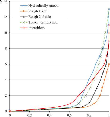
Рис. 10. Эпюра распределения скорости в у - u / U координатах
Fig. 10. Velocity distribution diagram in y - u / U coordinates
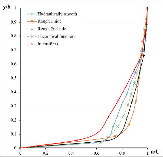
Рис. 11. Эпюра распределения скорости в y /δ- u / U координатах
Fig. 11. Velocity distribution diagram in y /δ- u / U coordinates
An analysis of the graphs and tabulated data shows that the presence of roughness significantly alters the shape of the velocity profile in the boundary layer compared to the hydraulically smooth case. A decrease in the boundary layer thickness is observed for rough surfaces. The velocity profile for the plate with intensifiers exhibits the most significant deviations, indicating a strong influence of macroscopic protrusions on the flow structure.
Analysis of measurement errors of the velocity distribution diagram in the boundary layer
To assess the reliability of the results, the absolute and relative measurement errors of the speed were calculated, taking into account the accuracy of the differential pressure gauges [5]. The results of the measurement error analysis for section No. 6 are presented in Tables 8 and 9.
The calculation of errors will be carried out according to the following dependencies:
u =

where Δ p – total pressure drop; ρ – density.
Let's take the derivative of this formula:
5 u =
f du
I d ( A P )
•5 ( A p ),
-1
du | 1 f 2 A p | 2 2 1
---- = — --- — = —, -.
I d (Ap) J 2 ^ p J p 2 -p-Ap
In its final form, we will write down the formula for finding the measurement error
5 u =
4 2 -P-A p
5(Ap) -5(Ap) = ^==-42-P-Ap
To find the relative error, we write:
δu 1 δ(Δp) =⋅ u 2 Δp where δ(Δp) –absolute error of pressure measurement.
Let us determine the absolute measurement error from the technical characteristics of the differen tial pressure gauge type HT-1890:
– accuracy of measurements at 25 оС: ±0,3 %;
– resolution 0.01 kPa;
– measurement range ±13.79.
Then the full measurement range is 27.58 kPa. The absolute error will be ±82.74 Pa.
As an example, we will provide the data obtained when calculating the errors of section 6.
Table 8
Results of the calculation of the measurement error for determining the velocity in the boundary layer, depending on the distance from the surface of the flow around the plate
|
Mm, from the plate |
Hydraulic smooth channel |
Rough plate, 1 side |
Rough plate, 2 side |
Plate with intensifiers |
|
0.5 |
±3.8 |
±2.82 |
±2.98 |
±4.49 |
|
1 |
±3.23 |
±2.46 |
±2.62 |
±3.29 |
|
2 |
±3.08 |
±2.30 |
±2.47 |
±2.9 |
|
3 |
±2.94 |
±2.24 |
±2.37 |
±2.62 |
|
4 |
±2.82 |
±2.19 |
±2.27 |
±2.41 |
|
5 |
±2.68 |
±2.14 |
±2.21 |
±2.24 |
|
6 |
±2.59 |
±2.09 |
±2.14 |
±2.11 |
|
7 |
±2.48 |
±2.12 |
±2.06 |
|
|
8 |
±2.39 |
±2.09 |
±2.02 |
|
|
9 |
±2.32 |
±2.08 |
±2.01 |
|
|
10 |
±2.28 |
|||
|
11 |
±2.26 |
|||
|
12 |
±2.26 |
|||
|
13 |
±2.24 |
Table 9
Results of calculating the relative error in determining the velocity in the boundary layer, depending on the distance from the flow surface of the plate
|
Mm, from the plate |
Hydraulic smooth channel |
Rough plate, 1 side |
Rough plate, 2 side |
Plate with intensifiers |
|
0.5 |
20 % |
11 % |
12 % |
29 % |
|
1 |
14 % |
8 % |
9 % |
16 % |
|
2 |
13 % |
7 % |
8 % |
12 % |
|
3 |
12 % |
7 % |
8 % |
10 % |
|
4 |
11 % |
7 % |
7 % |
8 % |
|
5 |
10 % |
6 % |
7 % |
7 % |
|
6 |
9 % |
6 % |
6 % |
6 % |
|
7 |
8 % |
6 % |
6 % |
|
|
8 |
8 % |
6 % |
6 % |
|
|
9 |
7 % |
6 % |
6 % |
|
|
10 |
7 % |
|||
|
11 |
7 % |
|||
|
12 |
7 % |
|||
|
13 |
7 % |
Analysis of functions describing the velocity profile of a boundary layer
In order to determine the hydrodynamic parameters of pressure losses in a section, as well as heat transfer in the ducts from the results of the experimental study on the formation of the boundary layer, it is necessary to approximate the results of the experimental study of the mathematical function necessary for further use in solving the equations of the dynamic boundary layer and energy balance [19].
Let's give an example for determining the functional dependence. For analysis, we will consider section No. 6 for a hydraulically smooth surface. When determining the dependence function — = f I У I dy we use a power function of the form (Table 10) U k§J
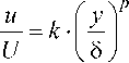
Table 10
Data for analysis
|
y 5 |
u U |
ln δ y |
ln u U |
|
0.03 |
0.63 |
–3.25 |
–0.44 |
|
0.07 |
0.72 |
–2.56 |
–0.31 |
|
0.15 |
0.75 |
–1.87 |
–0.27 |
|
0.23 |
0.78 |
–1.46 |
–0.23 |
|
0.3 |
0.81 |
–1.17 |
–0.2 |
|
0.38 |
0.85 |
–0.95 |
–0.15 |
|
0.46 |
0.87 |
–0.77 |
–0.12 |
|
0.53 |
0.91 |
–0.61 |
–0.09 |
|
0.61 |
0.94 |
–0.48 |
–0.05 |
|
0.69 |
0.96 |
–0.36 |
–0.03 |
|
0.76 |
0.98 |
–0.26 |
–0.015 |
|
0.84 |
0.99 |
–0.16 |
–0.007 |
|
0.92 |
0.99 |
–0.08 |
–0.007 |
Based on the experimental studies and processing of the obtained data, approximation functions were determined to account for the dynamic boundary layer distribution in various sections. Data for all studied surfaces were processed in a similar manner. The final approximation functions for all sections are presented in Table 11; the calculation using the approximation functions for section No. 6 is presented in Table 12.
Distribution functions of the dynamic boundary layer in different areas
Table 11
|
№ |
Smooth plate |
Rough plate, 1 side |
Rough plate, 2 side |
Plate with intensifiers |
Theoretical dependence |
|
3 |
1 — = 1.034 f У 1 735 и {5) |
1 — = 1'0356 .f У 1 1"42 U {5) |
1 — = 1.03037 .f У 1 12Л3 U {5) |
1 — = 1.06825 .f У 1 4'32 U {5) |
1 — -f У 1 7 и 4s) |
|
4 |
1 U _ f У 1 8'5 и Чз) |
1 15.49 — = 1'01679 • y U {5) |
1 14.2 — = 1.01302 • y U {5) |
1 8.13 — = 1.02422 • У и {5) |
|
|
5 |
1 U f y 1 6.2 u {5) |
1 15.49 — = 1.01679 • y U {5) |
1 — = 1.04288 .f У 1 734 и Ш |
1 3.7 — = 1.04378 • У U {5) |
End of table 11
|
№ |
Smooth plate |
Rough plate, 1 side |
Rough plate, 2 side |
Plate with intensifiers |
Theoretical dependence |
|
6 |
1 u ^ y I 7.18 U |
1 —- = 1.00691 .f У У12 U {8) |
1 9.08 — = 1.01032 . y U {8J |
1 U ( vV-57 — = 1.0279-| y I U <8) |
|
|
7 |
1 u -f У ^ 8.1 U |
1 u = 1.01563 .f У U {8 J |
1 —- = 1.02494 .f У I 7.91 U {8J |
1 и (vV.66 — = 1.01572 .| y I U {8) |
Table 12
Calculation result using approximating functions, section No. 6
|
Smooth plate |
Rough plate, 1 side |
Rough plate, 2 side |
Plate with intensifiers |
Theoretical dependence |
|
1 U f y |7.18 u - Us) |
1 — = 1.00691 .f У I1"12 U {s) |
1 9.08 — = 1.01032 .| y I U {8) |
1 U ( vV-57 — = 1.0279 .| y I U {8) |
1 — =f y 17 U {s) |
|
0.72 |
0.8 |
078 |
0.62 |
0.71 |
|
0.79 |
0.85 |
0.84 |
0.72 |
0.79 |
|
0.84 |
0.89 |
0.88 |
0.78 |
0.84 |
|
0.88 |
0.91 |
0.91 |
0.84 |
0.87 |
|
0.9 |
0.94 |
0.93 |
0.88 |
0.9 |
|
0.93 |
0.95 |
0.95 |
0.91 |
0.92 |
|
0.95 |
0.97 |
0.97 |
0.95 |
0.95 |
|
0.96 |
0.98 |
0.98 |
0.97 |
0.96 |
|
0.98 |
0.99 |
0.99 |
1 |
0.98 |
|
1 |
1 |
1.01 |
1.02 |
1 |
For section No. 6, a graphical dependence is presented for the velocity distribution diagrams in dimensionless y /δ- u / U coordinates for a hydraulically smooth plate, a rough plate (side 1), a rough plate (side 2), and a plate with intensifiers. The final approximating functions for section No. 6 are presented graphically in Fig. 16.
The obtained velocity profiles form the basis for subsequent calculation and analysis of hydrodynamic resistance and heat transfer coefficients, which are critical for the design of liquid propellant rocket engine cooling ducts.
Analysis of the obtained data (Tables 3–7, Figs. 10–11) demonstrates the significant influence of roughness, characteristic of SLM technology, on the kinematic structure of the boundary layer. It was found that for rough surfaces, the dynamic boundary layer thickness (δ) decreases. This phenomenon is explained by the intensification of turbulent mixing in the near-wall region of roughness protrusions, which generate additional flow turbulence.
The plate with intensifiers exhibits the most significant deformation of the velocity diagram, indicating strong interaction between the flow and the applied elements. From a practical standpoint, this means an increase in the local friction coefficient and, consequently, an increase in hydraulic pressure losses in the cooling channel. On the one hand, this requires increased pump power to pump the coolant, but on the other, it intensifies heat transfer.
The experimental data obtained were approximated by a power law (Table 11, Fig. 12). The exponent value obtained for a smooth surface agrees well with known data for a turbulent boundary layer (the "1/7 law"). For rough surfaces, an increase in the exponent is observed, indicating a more "filled" velocity profile closer to the wall.
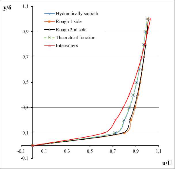
Рис. 12. Эпюра распределения скорости аппроксимированы степенной зависимостью в y /δ- u / U координатах
Fig. 12. The velocity distribution plot is approximated by a power dependence in y/δ-u/U coordinates
A key practical result is the derivation of specific exponent values for various types of additive surfaces. These data allow for direct refinement of hydrodynamic drag calculations in liquid-propellant rocket engine cooling channels, using modified friction laws that account for roughness. Further, based on the Reynolds analogy, these same relationships can be used to refine the methodological approach to analyzing heat transfer calculations.
Conclusion
This study addressed the problem of experimentally investigating the influence of additively manufactured surface roughness on the formation of a dynamic boundary layer in a rectangular channel. The study was conducted for M≤0.3, which did not require consideration of the compressibility of the working fluid. An experimental methodology was developed and described, including the design of the rig, the fabrication of test specimens with controlled roughness, and the pneumometric measurement technique.
The obtained results clearly demonstrate that the microrelief characteristic of parts created by selective laser melting has a statistically significant effect on the flow structure in the spatial boundary layer. It was found that roughness leads to a decrease in the thickness of the dynamic boundary layer and a change in the shape of the dimensionless velocity profile compared to a smooth surface.
The practical significance of this work lies in the identification of approximating relationships for the velocity profile, which can be directly used in refined mathematical models for calculating hydrodynamic drag and heat transfer in liquid-propellant rocket engine cooling ducts manufactured using additive manufacturing methods. This will improve the accuracy of design calculations and optimize designs by taking into account the actual properties of surfaces rather than idealized assumptions. Prospects for further research include conducting thermal experiments to determine the effect of the studied surface types on heat transfer, as well as numerical flow simulations using the obtained experimental data to verify the computational models.
