Exploring the Effect of Imaging Techniques Extension to PSO on Neural Networks

Published Online April 2020 in MECS DOI: 10.5815/ijigsp.2020.02.02

The main purpose of all metaheuristic algorithms is to explore the search space and help in reaching to the optimum or near-optimum solution. Some of the main problems that might not help the metaheuristic techniques to reach to optimum solutions is either because of the complexity of the problem or problem resources are unclear or limited [15]. Most of the metaheuristic algorithms are inspired and adopted from biology or nature such as chromosomes, birds, fish swarm and bats [10].

In nature, humans try to explore space through various tools such as telescopes, satellites and radars. Usually expeditions to discover the space are sent after very deep investigations through the previous mentioned tools. This will help in limiting the scope of exploration towards the scientist’s target. The closer the expedition to the target, the more effort will be done starting from the reached position. The general idea is to maintain randomness under control. Most of the metaheuristic techniques depend on randomness but usually randomness might lead to more cost in terms of time and resources. To reduce this problem, human expeditions move in a controlled randomness to ensure reaching to nearoptimum solution consume less cost.

Many researchers work to either propose new metaheuristic techniques inspired from biology or develop systems that combine various metaheuristic techniques. Proposing new techniques such as Genetic Algorithm (GA)[11], Simulated Annealing (SA) [17], ant colony [6,7], bat algorithm[31], PSO and fish swarm [16][26], and Combining more than one technique such as PSO and GA, GA and SA, or PSO and SA [4][12,13][27][31]. In both the cases, proposing new metaheuristic or combine more than one technique, the target is to better explore the search space and achieve better results (near-optimum).

In [22] Richards and Ventura proposed a technique to initialize the population called centroidal Voronoi tessellati which starts with a population that is generated randomly then iteratively tries make the particles move far from each other as possible to have a diversity in the initial population. In [21] authors proposed another technique for population initialization where the random particles are generated and with each generated particle its complement/inverse particle is also generated. Then from these particles the initial population is generated.

In [18] Maaranen et.al proposed a technique called quasi-random generator technique to initialize the population. This technique forms repetitive patterns to avoid having many particles in similar/close locations. This technique’s idea is based on generating a population with high diversity as possible.

Based on the researchers work, they try to have a diverse initial population which means having diverse particles so that they can capture the most of the good particles. However, this might not always true because this might be done regardless of the importance of these particles. The imaging technique depend basically on exploration first then expedition, which means checking first the potential particles then forming the population.

Initialize swarm

Do until maximum iterations or minimum error criteria

For each particle

Calculate location’s fitness value

If the fitness value is better than pBest

Set pBest = current fitness value

If pBest is better than gBest

Set gBest = pBest

For each particle

Calculate particle’s new velocity and location

End Do until

Fig. 1. Particle swarm optimization pseudo code; pBest: Best solution found by particle, gBest: Best solution found by swarm [28]

In this research, our objectives is to explore the effect of imaging techniques as extend to PSO in the classification of neural networks. We are not interested to compare the obtained results with other approaches, but instead we care about comparing the obtained results using extend PSO and the regular PSO. To evaluate imaging techniques, they are implemented to extend a particle swarm optimization metaheuristic used to tune the weights and biases of multiple classification neural networks in seven different datasets. Thus, the following three subsections briefly introduce the particle swarm optimization metaheuristic and the artificial neural network techniques.

• A.    Particle Swarm Optimization

PSO is a very well know metaheuristic search algorithm used in various applications ranging from science, business, optimization to engineering [14][27][31][32]. The idea of the algorithm has been inspired from the movements and travel of birds. The main steps of the algorithm is illustrated in Fig. 1. Each bird in the bird’s flock represents a particle and in each algorithm iteration the velocity and the location of each particle is updated. For more details about concepts of PSO, researchers can refer to [16][26]. As will be explained in the next sections PSO is selected to be our metaheuristic technique.

• B.    The neural network

Artificial Neural Networks (ANN) are an active area of research in the fields of artificial intelligence and machine learning invented as techniques to loosely mimic the function of neurons in living beings.

Applications of the neural network such as classification require configuring a set of parameters called the weights and biases of the network so that for a given set of inputs describing some object, the neural network could produce a correct output identifying that object. Several algorithms such as the back-propagation algorithm can be used to perform the task of configuring/training the network [24]. In this paper we use imaging techniques as extension to metaheuristic technique (i.e., PSO) to explore their effectiveness in improving the accuracy of neural network classification.

• C.    Metaheuristic Approaches for ANN

Backpropgation (BP) algorithm is a very well known algorithm used in feed farward ANN training. Training using BP may yield some times to what so called local minima which prevents reaching to global minma and the training does not improve [13]. Various techniques and methods have been tried to get rid of local minima, some of these are using metaheuristic techniques. Many researches have been working to adjust the neural networks weights based on methaheuristic techniques to improv the classification, some of these are based on GA and PSO as examples [12][19]. In other cases, reserchers attempt to combine more than one metaheuristic approach to utilize the capabilities of each one of them, therefore, trying to obtain better classification accuracy than using one technique alone [12,13]. In this paper we select PSO as a well defined metaheutstic technique that has been used in improving the neural network classification as a technique to be extended by imaging techniques to measure the effectiveness of those imaging techniques in improving the neural network classification

• II.    Imaging Techniques

In this section we present briefly some of the imaging techniques that were proposed by Abbas and Hewahi [1]. These imaging techniques work as a telescope to gather information first about the search space then help the metaheuristic technique to direct its search. This process will be continuously performed throughout all the searching stages (during initialization or during the main search) within the metaheuristic algorithm. To understand the imaging techniques, we need first to define what we mean by image. Imaging techniques in [1] have been tested on multiple optimization functions using COCO and have shown a good potential to improve the results.

• A.    The image

Image in imaging techniques concept means capturing a certain area in our search space. This captured area should be bounded and we refer to that by scope. The image has resolution which means the number of pixels, here those pixels are referred to be as temporary particles. When the image is taken within a certain scope, its pixels will be checked against their usefulness based on the used imaging technique, if useful, they will be within the population and if not, they will be discarded. Every pixel has a fitness value and based on that it will be preserved and added to the population or discarded [1]. The imaging technique can be merged to a metaheuristic search as shown in Fig. 2. Fig. 3 shows the extend PSO. Capturing images (pixels) in the Figures mean instantiating several particles within a certain range but without still considering them as particles. The image technique then selects some of these to create the initial population. Similar thing will be done during the main search by selecting certain pixels to be temporary particles and then based on that the population will be updated. The temporary pixels will be then discarded.

Generally, the more is the number of temporary particles/pixels, the better is the captured area of the search space.

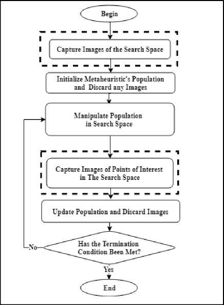
Fig. 2. General metaheuristic imaging extension flowchart

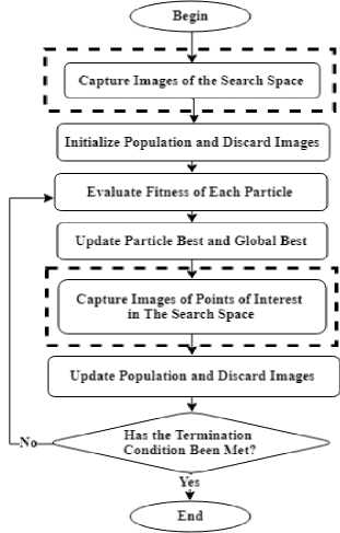
Fig. 3. PSO imaging extension flowchart

• B.    Imaging Types

In this research we present various imaging techniques that can be incorporated with any metaheuristic algorithm which starts from initial population. We consider five types, out of which four are used during the initial population and one used during the main search. The four used for the initial population are Starry Night (SN),

Fireworks (FW), Lanterns (LN) and the Grid (GRD). The first three imaging types are given in [1], whereas the fourth one is a new proposal, The fifth imaging type is used during the main search and called Connecting the Dots (CDT) [1].

• •    Starry night

This technique is applied during the generation of the initial population generation. Fig. 4 shows the SN mechanism.

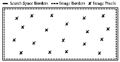
Fig. 4. Starry night (SN) imaging technique

Starry night technique is quite simple in a way that one global image represents the search space and as many as possible number of pixels are generated. For every generated pixel, a fitness value is computed. Those pixels with high values are selected to form the initial population and the rest will be ignored. One major parameter in this technique is the number of generated pixels in the scope of the image [1].

• •    Fireworks

This technique is applied during the generation of the initial population generation. Fig. 5 depicts the mechanism of FW.

^ Search Space Borders ---Image Borders X Image Pixels

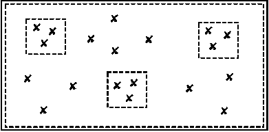
Fig. 5. Fireworks (FW) imaging technique

This technique can be summarized as below:

• a.    Follow the same procedure used in SN by having one global image and generation of pixels.

• b.    Create some equal sized local images within the scope of the global image.

• c.    Form the population from the best pixels in the local images and the global image.

As done with SN technique for every pixel a fitness value is obtained and then those with the best values are selected as the initial population and the rest will be ignored. In this technique we have several parameters such as number of pixels in the scope of the global image, number of pixels in the scope of local images and number of equal sized local images [1].

• •    Lanterns

This technique is applied during the generation of the initial population generation. Fig. 6 shows the mechanism of LN.

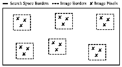
Fig. 6. Lanterns (LN) imaging technique

In this technique no global image is captured first but instead many local images with equal sized are taken. The fitness value for every pixel is computed then those pixels from the local images form the population. Parameters necessary for this technique are number of local images (scopes) and number of pixels in each the local image [1].

• •    The grid

This technique is used in initial population generation. Fig.7 shows the mechanism of GRD.

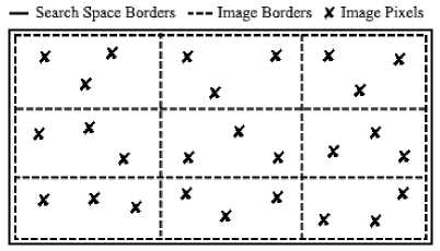
Fig. 7. The grid (GRD) imaging technique

The Grid technique is a bit more elaborate than the past introduced techniques. In this technique the search space is divided up into as many equally sized zones as possible and full scope images of each zone are captured. The biggest limitation to this technique is the number of dimensions, since the number of zones resulting from bisecting every dimension would exponentially increase. Because of that, the technique was modified to accept as an input a random number of dimensions to bisect instead of bisecting every dimension in the search space. For each image captured, an average of the fitness value of pixels inside each zone is calculated, with the resulting average made to represent the quality of zone. After that, pixels from the best zones were used to initialize the population and the rest were discarded. The main parameters of this technique are number of dimensions to bisect, number of zones which is equivalent to 2n, where n is the number of dimensions to bisect, and number of pixels to generate per zone image.

• •    Connecting the dots

This technique is applied during the main search or what so called during exploration phase. Fig. 8 depicts the CDT technique [1].

— Space Borders ---Image Borders X Pixels «Particles

2Г”L

1                     ।

Xi Л i- *

iT_____

Fig. 8. Connecting the dots (CDT) imaging technique

In this technique the used population is to be updated, the process starts by choosing the best particles from the population and then around each of these particles a local image is formed given that the selected particle location is the center of the image. Specifying the selected particles, pixels around each of the center particle within the image scope are generated and the fitness value for each is calculated, if any pixel within the image is having a better fitness value than the particle, the new pixel will be the center of a new image and it replaces the old particle in the population. The low-quality pixels will be ignored. Parameters involved in this technique are number of the best particles to be selected and number of pixels to be generated around the particle.

• III.    The Experimentation

As a case study, the imaging techniques coupled with PSO as a metaheuristic technique are used to tune ANN weights and biases for multiple neural networks trained against several datasets. Following, is a description of the conducted experiments.

• A.    The datasets

In this research, multiple datasets with varying numbers of records, input attributes, and output objects to classify are utilized. In total, there are seven datasets which were obtained from the popular UC Irvine’s machine learning repository [8].

The datasets are formatted as csv files where each row contains a set of input attribute values and a class output identifying that object. Table 1 highlights the basic information related to these datasets.

Table 1. Datasets basic information[8]

Dataset	# Attributes	# Classes	# Instances
Iris	4	3	150
Seeds	7	3	210
Glass	9	6	214
Zoo	16	7	101
Yeast	8	10	1484
Cars	7	4	1728
Landsat	36	6	6435

• B.    Experiment methodology

The imaging techniques are to be used to gather information about the search space and support the search effort of a given metaheuristic during the phases of population initialization and the main search phase as shown in Fig. 9. In this research the imaging techniques are used to support PSO in tuning the weights and biases of a set of neural networks trained as classifiers for several datasets. Fig. 10 demonstrates how the imaging techniques are integrated with PSO.

In total, 10 scenarios were formulated for benchmarking and comparison, these are:

• 1)    Apply none of the imaging techniques (i.e. only apply PSO to train the network), this is referred to as the “Regular” case.

• 2)    Apply SN

• 3)    Apply FW

• 4)    Apply LN

• 5)    Apply GRD

• 6)    Apply CDT

• 7)    Apply SN and CDT

• 8)    Apply FW and CDT

• 9)    Apply LN and CDT

• 10)    Apply GRD and CDT

The evaluation of the results is carried as follows: For the criterions of training dataset classification accuracy, test dataset classification accuracy, and training runtime, each scenario is benchmarked for a total of 20 times per dataset and the accuracy scores for each dataset is averaged separately. These averages will be considered as the final scores for the scenario. In the end, the three criterions results for each scenario is compared to the rest of the other scenarios per dataset as well as the overall performance of each across all datasets.

• C.    Experiment parameters

In this section, the parameter values for each of the elements in the experiment are presented.

Before commencing, it needs to be mentioned that the codebase is derived from the work of McCaffrey [19]1 9 ] on a tutorial explaining how to apply PSO on neural networks to solve a classification problem of a subset of the Iris dataset (30 records), and that several parameters from the original codebase were maintained such as PSO’s inertia, personal and social weight parameters.

• •    PSO parameters

• -    Number of particles: 50

• -    Number of iterations: 100

The above parameters basically result in allowing PSO a total of 5000 examined solutions in the search space, which should give PSO at least some chance to explore the search space.

• -    Inertia weight: 0.729

• -    Personal weight: 1.49445

• -    Social weight: 1.49445

With the Personal and Social weights discussed in section I-A being equal, PSO would give equal importance to acting cooperatively to explore the search space as well as independently.

• •    Neural network parameters

Th neural network parameters are: the input layer number of inputs, number of hidden layers which was limited to one, number of neurons per hidden layer, and number of neurons in the output layer. These parameters will vary from one dataset to another depending on the number and type of input attributes, as well as depending on the number and type of possible output classes.

The listed parameters determine the number of dimensions in the search space as follows:

Number of dimensions = (Number of inputs * Number of hidden layer nodes) + (Number of hidden layer nodes *

Number of out-put layer nodes) + Number of hidden layer nodes + Number of output layer nodes                 (1)

Table 2 presents the parameter values used for each dataset.

Table 2. Neural network dataset parameters
Dataset	Dataset Size (N.O. Records)	Inputs	Hidden layer nodes	Output layer nodes
Iris	150	4	6	3
Seeds	210	7	6	3
Glass	214	9	7	6
Zoo	101	16	9	7
Yeast	1484	8	6	10
Cars	1728	11	6	4
Landsat	6435	36	4	6

One further note, when a dataset is loaded into the program its records are randomized and split 70% to be used as a training dataset and 30% to be used as a test dataset.

• •    Imaging techniques’ parameters

  To keep things somewhat even, the parameters were selected on the basis that the use of any of the proposed imaging techniques (SN, FW, LN, GRD, CDT) would yield a total of around 500 pixels or temporary particles. And to compensate for the overhead resultant from using these imaging techniques, an extra 10 iterations were added to the “Regular” scenario, denoted by R-110, when benchmarking against single imaging technique scenarios (10 iterations * 50 particles in population per iteration = 500 particles), and an extra 20 iterations were added to the “Regular” scenario, denoted by R-120, when benchmarking against dual imaging technique scenarios where two imaging techniques are applied (20 iterations * 50 particles in population per iteration = 1000 particles).

In Table 3, the parameter values for each imaging technique are presented. These parameters were selected based on some trial and error and should be suitable for the experiment.

• IV. Experiment Results And Analysis

In this section, the results of the experiments related to each dataset are shared in terms of training data accuracy results, test data accuracy results and program runtimes. Each dataset has been used for 20 times with every scenario, and the average of these runs has been taken as the scenario performance using that dataset.

Table 3. Imaging technique parameters

Technique	Parameters	Total Pixels
SN	No. global scope image pixels: 500	500
FW	No. global scope image pixels: 400 No. local scope images: 20 No. pixels per local image: 5 local images radius as a percentage of dimension size: 5% of the search space	500
LN	No. local scope images: 100 No. pixels per local image: 5 local images radius as a percentage of dimension size: 5% of the search space	500
GRD	No. dimensions to bisect: 8 No. zones: 2^8 = 256 No. pixels per zone image: 2	512
CDT	No. PSO particles to apply the technique on: 1 No. pixels to generate around each particle: 5 local images radius as a percentage of dimension size: 5% of the search space	500

A. Training data accuracy results

For the training, the imaging techniques have overall produced better results than both regular cases R-110 and R-120. Fig. 12 and Table 4 summarize these results.

FW seems to have performed best during the training phase of the neural network both when used alone as well as when combined with CDT, which shows the effectiveness of an imaging technique that combines global imaging of the search space with local images of promising areas in the global image simulating the zooming effect of a telescope.

The best results overall were scored using the FW+CDT dual imaging technique, which demonstrates the effectiveness of the use of imaging techniques during both the phases of population initialization and during the main phase of the metaheuristic.

The worst overall scores in both single and dual imaging technique scenarios were scored by R-110 and R-120. In fact, R-120, intended for comparison against dual imaging techniques, was even outperformed by single imaging technique scenarios. This demonstrates how the use of any imaging technique could perform better than not using any. And, the average of R-110 was also marginally better than R-120 which might demonstrate that when relying only on PSO and on random initial populations it does not guarantee better training accuracy scores even with the additional 10 iterations in R-120.

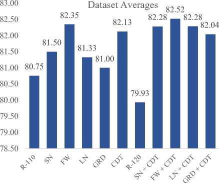
Fig. 12. Overall dataset training data accuracy results(%).

• B.    Test data accuracy results

For the testing, overall, the imaging techniques have produced better results than both regular cases R-110 and R-120. Fig. 13 and Table 5 summarize these results.

It has been noted that each of the dual techniques performed better than the corresponding single technique (e.g., GRD+CDT is better than GRD alone), which indicates the importance of CDT to improve the performance. An additional noted remark is that FW has again scored best as a single imaging technique, which is consistent with the previous training dataset accuracy scores and shows the effectiveness of this imaging technique. However, GRD+CDT has scored best in the case of dual imaging technique scenarios.

Still, the difference in accuracy between the first three top approaches was minor (i.e., the difference between the lowest and highest is 0.57) an the shift in the order of some scores between the training phase and the testing phase is not necessarily unexpected since it could be influenced by such things as the quality of the datasets used and the disparity between the data in the training datasets and the test datasets. The worst scores in both single and dual imaging technique scenarios were again scored by R-110 and R-120. Again, R-120, intended for comparison against dual imaging techniques, was even outperformed by all single imaging technique scenarios. This demonstrates how the use of any imaging technique could perform better than not using any, and since R-110 had overall better accuracy scores than R-120 in the training phase, it has again produced better scores in the testing phase.

Table 4. Datasets training data accuracy results summary(%)

Data	R-110	SN	FW	LN	GRD	CDT
Iris	100.00	100.0	100.0	100.0	00.00	100.0
Seeds	97.59	97.52	97.93	98.19	97.49	98.53
Glass	69.33	71.41	71.36	69.27	69.57	71.77
Zoo	87.89	91.34	92.76	88.59	88.94	90.14
Yeast	49.70	50.33	51.42	51.69	51.59	52.51
Cars	82.78	83.17	84.05	84.19	83.07	83.64
Land	78.00	76.70	78.92	77.40	76.36	78.30
Avg	80.75	81.50	82.35	81.33	81.00	82.13
Dataset	R-120		SN + CDT	FW + CDT	LN + CDT	GRD + CDT
Iris	99.42		100.0	100.0	100.0	100.00
Seeds	97.97		98.46	98.88	97.90	98.09
Glass	67.93		70.39	71.54	70.97	70.87
Zoo	87.02		90.22	91.05	91.98	88.60
Yeast	50.10		51.01	51.43	52.14	51.36
Cars	82.05		85.81	85.64	84.56	85.02
Landsat	75.03		80.10	79.11	78.45	80.37
Avg	79.93		82.28	82.52	82.28	82.04
Table 5. Datasets test data accuracy results summary(%)
Data	R-110	SN	FW	LN	GRD	CDT
Iris	91.65	91.87	92.09	91.65	91.87	91.33
Seeds	91.61	91.61	92.01	90.50	91.30	91.93
Glass	58.45	60.47	58.83	58.66	59.06	59.45
Zoo	79.84	82.50	82.17	79.00	80.66	80.01
Yeast	43.85	44.64	44.47	45.99	45.61	46.39
Cars	77.13	78.07	78.46	79.63	77.54	78.04
Land	76.52	74.99	77.48	76.02	74.86	77.10
Avg	74.15	74.88	75.07	74.49	74.41	74.89
Data	R-120	SN + CDT		FW + CDT	LN + CDT	GRD + CDT
Iris	91.67		91.87	91.76	91.10	91.65
Seeds	91.22		92.25	91.30	90.90	91.77
Glass	56.48		58.51	59.77	59.21	58.82
Zoo	80.50		82.17	80.67	80.34	84.67
Yeast	44.18		45.40	45.40	46.06	45.12
Cars	76.64		80.35	80.04	78.52	79.37
Land	73.43		78.98	77.71	77.34	79.20
Avg	73.44		75.65	75.23	74.78	75.80

• C.    Runtime Results

76.00 75.50 75.00 74.50 74.00 73.50 73.00 72.50 72.00

The program runtimes (representing the average neural network training time over the course of 20 runs per scenario) were perhaps harder to gauge since they may be affected by such factors as code efficiency and machine performance hiccups and that could cause some minor noise in runtime scores.

Dataset Averages

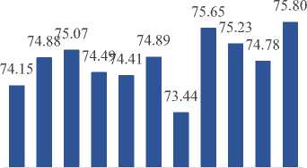
Fig.13. Overall dataset test data accuracy results(%).

Still, the imaging techniques were noted generally to have achieved better runtimes than their regular technique scenario counterparts across all datasets with some exceptions. Fig. 14 and Table 6 summarize these results. The trio of SN, FW and LN have scored the best runtime scores both when used alone as well as when combined with CDT achieving similar results due to their similar implementations. This demonstrates that these imaging techniques are less costly to use in addition to tending to produce better results when compared to the regular case of using PSO alone. In contrast GRD and CDT on average did not perform better than R-110 and R-120 but were marginally close.

Dataset Averages

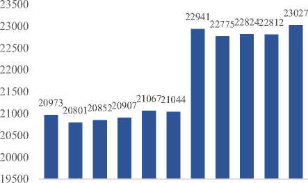
Fig. 14. Overall dataset training runtimes (milliseconds)

• V. Research Conclusions And Future Work

This research proposed the idea of imaging the search space to gather information about that space and support the search effort of a given metaheuristic during the phases of population initialization and the main search phase. Furthermore, a set of basic experimental imaging techniques were devised, four of which are used during the initialization phase of a metaheuristic, namely starry night (SN), fireworks (FW) lanterns (LN) and the grid (GRD). The fifth technique (CDT) is used during the main search phase of a metaheuristic. SN is based on taking a single global scope image of the search space that is as high resolution as possible. FW is based on taking a single global scope image of the search space followed by several localized images around points of interest from the global image. LN is based on taking localized images all over the search space. GRD is based on dividing the search space into several equally sized zones and capturing images of these zones. CDT is based on incrementally taking several images with the first image being revolved around some particle in the PSO population and the following images being revolved around any pixel with better quality.

To validate the idea and evaluate the devised imaging techniques, the techniques have been applied on a particle swarm optimization metaheuristic used to tune the weights and biases of multiple neural networks trained to classify objects found in a total of seven different datasets (The iris dataset, the seeds dataset, the glass dataset, the zoo dataset, the yeast dataset, the cars dataset and the landsat dataset) and the performance of the imaging techniques was compared to the use of PSO alone to train the neural networks, both when each of these techniques is used alone (single imaging technique scenarios) as well as when any of the initialization imaging techniques SN, FW, LN, or GRD are combined with the main phase.

The experimentations show that the imaging techniques demonstrate better performance than only using PSO alone in terms of training and testing accuracy of the results vs the runtime cost of applying these techniques. However, perhaps in part due to the simplicity of the experimental imaging techniques, the improvements were not too significant and repeated experiments did not guarantee consistent results every time. Among the techniques, it seems that the FW imaging technique or FW+CDT is best since it combines elements of global imaging and local imaging for a zooming effect on points of interest like that of a telescope. It is to be noted, despite that FW did not outperform the other techniques all the time, it has done well in most of the cases which makes it suitable for a wide range of problems. For future work, there are many research possible directions related to the proposed concept of imaging such as developing new imaging techniques (e.g. developing a negative imaging technique inspired by the opposite based learning technique),

Table 6. Datasets runtime summary (milliseconds)

Data	R-110	SN	FW	LN	GRD	CDT
Iris	1318	1335	1317	1314	1337	1327
Seeds	1970	1951	1949	1937	1962	1960
Glass	2960	2944	3018	2940	2971	2959
Zoo	2199	2182	2183	2212	2208	2194
Yeast	21790	21683	21718	21708	21907	21930
Cars	18823	18668	18660	18692	18880	18843
Landsat	97754	96842	97123	97547	98205	98094
Avg	20973	20801	20852	20907	21067	21044
Data	R-120	SN + CDT		FW + CDT	LN + CDT	GRD + CDT
Iris	1424	1424		1418	1463	1433
Seeds	2081	2094		2075	2063	2104
Glass	3206	3203		3210	3197	3227
Zoo	2421	2373		2370	2403	2400
Yeast	23909	23728		23710	23729	23927
Cars	20417	20464		20439	20393	20606
Landsat	107128	106141		106544	106436	107490
Avg	22941	22775		22824	22812	23027

extending the basic techniques presented in this research with more advanced ideas (e.g. developing a version of FW that incorporates multiple zoom levels on points of interest in the search space), developing new ways to utilize the presented imaging techniques (e.g. applying SN,FW or LN during the main search phase of a metaheuristic instead of during initialization), benchmarking the presented techniques against problems other than that of tuning a neural network, and extending metaheuristics other than PSO with the presented imaging techniques.