Extended Probabilistic Cost Model (EPCM): A Framework for Cost Estimation of Wireless Network Deployment in Rural Areas

Published Online January 2017 in MECS DOI: 10.5815/ijieeb.2017.01.01

Wireless Networks have been presented as an appealing solution to bridge the digital divide between rural and urban regions. This is due to their ease of deployment and the ever-decreasing cost of the technology. The design and the deployment of wireless networks have gained attention from researchers. Many problems tied to those networks have been addressed, such as routing protocols, channel assignment, and topology design, especially in wireless mesh network.

The design of wireless network has been usually capacity-driven, meaning that the main concern is the capacity in terms of throughput and/or delay. This design approach is more tied to urban regions where a return on investment can be easily ensured. In contrary, the design of the network should be cost-driven in rural regions; because it should meet a compromise between the low affordability of the population and the minimum required capacity. In this configuration, an underestimation or overestimation of the overall cost, usually observed in deployments, can be very harmful to the project.

Some strategic projects have been abandoned during their deployment (15 % in 2010) [2] because of lack of funds, which results from a poor cost estimation.

However, to estimate the cost of a wireless network deployment is not a trivial task; because of variations in the cost of equipment and the arrival of unexpected events during deployment [9]. To solve this problem, several models have been developed, including the Fuzzy analogy [18], the Automata Neural Network (ANN) [17] and the Probabilistic Cost Model (PCM)[10].

Although PCM is one of the latest models and is more suitable to tackle this problem, it has also the same limitations; among which the consideration that every unexpected event influences the overall cost with the same intensity. Moreover, the average unexpected costs must be known in advance.

This work aims to provide a cost estimation framework for the deployment of a wireless network that attempts to fill the gaps of PCM model while taking contingencies into account.

To achieve this aim, we collected first information in various telecommunications companies in the city of Ngaoundere (CAMTEL, Orange, and MTN), including the initial estimated cost of each project, the number of days scheduled for deployment, the arrival times of unexpected events and the total cost of these events for each deployed project. We include also various unexpected events that may occur during the network deployment and their associated costs. We use therefore the Poisson process to predict the number of unexpected events that may occur during network deployment; we also take into account the probability that the total cost of these events does not exceed a given contingency.

This paper is organized as follows: A review on the network cost estimation models is presented in Section 2, the third section describes the proposed framework for the cost estimation of a wireless network in rural areas. Section 4 presents the results and discussions. The end provides an overall conclusion and outlook.

• II.    Related Work

Numerous studies have already tackled the problem of cost estimation for the deployment of a wireless network. In this section, we discuss existing models and show their limitations which triggered our investigation into an alternative method.

• A.    Fuzzy Analogy

The cost estimation of network goes through three steps [4]:

• 1.    Identification of deployment projects with a set of attributes.

• 2.   Evaluation of similarities between the new project

• 3.   Adaptation.

and other historical projects.

A.1. Project identification by a set of attributes

The objective of this step is to select the attributes that best describe the project and which are independent and meaningful to the cost estimation. For the significance test, for example, practice is to assess the correlation between each attribute and project cost. Thus, if the level of this correlation is satisfactory, the attribute is selected.

A.2. Evaluation of similarities between the new project and previous ones

It involves looking for similarities between projects. Indeed, projects are ordered according to their degree of similarity with the new project. In fuzzy logic, a similarity measure is a function of values in the range [0,1] denoted d(P1, P2) which evaluates the similarity between Pl and P2 projects based on d_Vj (P1, P2) which in turns evaluates the similarities between attributesV j of Pl and P2 projects. We get d_vj ( P l, P 2) d _V( (P1, P2) from the following formula [15]:

^max^min k ( p j P l), ц^

di Pl, P 2) = <

max - min aggregation Z k Ц a ( ^{P 1}) *ц / ^p 2)

sum - productaggregation

min max k

( l-ц ^( ^{P 1}), Ц ^( P 2) )

min - kleene - Dienesaggregation

Where d_V( (P1,P2) = Imeans the two projects Pl and P2 are perfectly similar according to Vj attribute; dyj (P1,P2) = 0 means that Pl and P2 are not similar;

0 < d „j (P1,P2) < Imeans that Pl and P2 are partially similar.

ц j are the membership functions representing fuzzy Ak sets and for each attribute we have linguistic values (fuzzy set). The membership functions establish an association betweeneach element of the set of cost and a real in [0,1].

A.3. Adaptation

The objective of this step is to deduct the estimated cost of thenew project , using costs of the deployment projects similarto , this by using the weighted average cost of all similarprojects. For this task we use the following equation:

C ( ^P ) =

Z N

d ( P , Pi ) X C ( Pi )

^N d ( P , Pi )

Where ( , ) is the estimated cost of the new project; is the new project; is a similar project to the new project in the given set; ( ) is the cost of the project and ( , ) are the membership functions which express the actual valueof the fuzzy proposition that and are similar.

The Fuzzy approach helpssolving problems in different areas. In [13] this approach is used to classify documents into appropriate clusters using the Fuzzy C Means (FCM) clustering algorithm. To quantify reusability, a fuzzy multi criteria approach is studied in [11]; this approach tackles the unpredictable nature of reusability attributes.

However the analogy Fuzzy has a big drawback, it fails to dealwith the uncertainties caused by the cost of dynamic changeduring the deployment of the project.

• B.    Artificial Neural Network

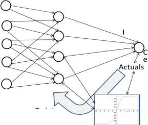
The method ANN (Artificial Neural Network)[7][8][5] minimizesthe error in the cost estimation using a dedicatedalgorithm to train neurons to respond to different situationsand new data miscellaneous costs. In this model, neurons areorganized into layers and each layer can have connections tothe next layer. Figure 1 shows an example of such a network for costestimation of network deployment. The network produces aresult (cost) by propagating its initial inputs (factors of costand project attributes) through the various neural networksto the exit. Each neuron of a layer computes its outputby applying its activation function according to its inputs.Generally, the activation function of a neuron is the sigmoidfunction defined by:

f ( X ) =------ (3)

1x

+ e

Neural Network is also used to analyse the vascular pattern recognition [12].

Data inputs

Estimation algorithms

(HiddenTayer)

AP costs

Testing

Labour cost

CPE costs

Deployment costs

APEX

Sigmoid function

Training algorithm

Fig.1. Automata neural network

Ы

P[C _tU e <  в ] = 2 P[C tue <  в I X = x ] P[X = x] x = 0

Model outputs

ы

^ P[Ctue < в] = 2Ф x=0

X x X e

— X

x !

^ p

Disadvantage: There is no standard approach to the choiceof different parameters of the topology of a neural network(number of layers, number of processing units (neuron), initialvalues of the connection weights, etc.).

C. Model PCM (Probabilistic Cost Model)

This model provides the probability that the cost of unexpectedevents do not exceed a certain threshold (contingency). Toobtain a cost estimation of unexpected events [9], we use:

n

C- = 2 C i           (4)

i = 1

Where Ci is the set of all the costs of unexpected eventsand C _{tu e} is the total cost of unexpected events. In this model, itis assumed that all costs of unexpected events follow a normaldistribution with even the same parameters. This mean

^Ci~^{N (} t c , ^ c ') ^ C_te~^{N (} n T c ^,n CT 2 )      (5)

Where p_c and a_c are respectively the mean and the standarddeviation of the range of costs for each unexpected event andn the number of unexpected events.

C.1. Probability of having cost overrun

The purpose of this subsection is to use the average costof unexpected events of deployment projects, the standarddeviation between the costs of unexpected events and theaverage rate of events per unit time, to find the probabilitythat the total cost of unexpected events do not exceed theestablished contingency.

Let X a number of unexpected events. If the estimator attachesa contingency P for the unexpected events, it will havea confidence rate percentage p against the estimated costoverruns as:

P[C tue <  PA ^ p                   (6)

Where C _tue is the total cost of unexpected events, p_c theaverage cost of unexpected events, X the average rate of arrivalof events, C = —is the coefficient of variation

Me changes dueto cost changes and Ф(z) is cumulative distribution functionof z , C is the initial cost of deployment.

C.2. Estimated cost of unexpected events

Let p_c the average cost of contingencies and Л the rate of unexpected events during the deployment period, a cost estimation of unexpected events such as the initial cost ratio is obtained as follows:

(

E ( Otue ) = E 12 Oil

V i=1

According to Benjamin and Cornell [1], we have:

E ( Otue ) = E ( X) E ( Oi)

Since the random variable X follows a Poisson distributionwith parameter Л, we have [14]:

E ( X ) = X and E ( O ) = ^^

C

Where:

C.             Ц

Oi= - ^ Oi~N (H , ^Tc-) C            CC

Thus from conditional distribution of O tue we have

C.nC

Otue = — ^ O^x=n ~ N(-^^, ^Tc-)

C                 CC

Limitations: This model is interesting but still has drawbacks:

• •    This model considers all the costs of unexpected events are normally distributed with same parameters (identical) and therefore similarly influence on the total cost of these events, which is not very realistic.

• •    We must first know the average cost of unexpected events which is considered as the cost of each event.

Table 1.Unexpected events

Event	Mean cost (FCFA)	Standard deviation (FCFA)
Temporary events
Construction of culvert toprevent the crossing of theriver	770000	423871.05
Expansion site enclosures	4258500	2456191.16
Armourstone slippedground	884500	506463.23
Pylon price variation	-12.5 %	3.54
Compensation crops	147033	59645.65
Need generator and diesel	(6000*T)+635 943.3	298245.86
Router prices change	-12.2 %	4.15
Controller prices change	-9 %	2.64
Antenna prices change	-12 %	4.36
Access point priceschange	-13.5 %	4.95
Field embankment afterdisasters	1273000	668923.01
Switch prices change	-13.5 %	4.95
Structural events
Repair community well	112500	17677.67
Repair collapsed wall	225000	145773.79
Damaged antenna
Moving an antenna	2250000	353553.39
Communal fees	264563	446.89
Damaged access point
Construction pens security	2025000	954594.15
Damaged Switch
Damaged router
Adding emergency cell	1994083	1480425.12
Moving and repair CDEnetwork	433333.33	225462.48
Moving and repair ENEOnetwork	1217166.67	665521.29
Damaged controller
Moving and repair AERnetwork	832500	38537.32
Deviation       of       water collectionnetwork	406085	59361.87
Moving WC on itinerary	112500	17677.67
Moving       and       repair privateelectricity network	832500	38537.32
Events related to standard
Transformation steady self-pylon in pylon guyed	6675000	3146625.18

• III.    Extended Probabilistic Cost Model(Epcm)

The PCM model (Probabilistic Cost Model) as describedpreviously is based on the determination of cost of unexpectedevents and the determination of the probability that the totalunexpected cost does not exceed a given contingency. Inthis model, an unrealistic consideration is made that all thevarious costs of unexpected events follow the same normaldistribution with the same parameters, i.e. the same averageand standard deviation meaning that these costs are equal.

This assumption is not very realistic because the probabilitythat all the unexpected events have distributions (possible setof each event) with the same average and the same standarddeviation is almost zero: These events are totally different. Inthis model, the author uses data from already deployed projectsto determine the cost of their unexpected events. It, therefore,raises the question of how to find the unexpected costs fornew deployment projects.

Unexpected events that occur during deployment arrive in arandom way, independent from each other, and only one eventoccurs at a time. The number of events depends on the durationof the deployment, so we can use the Poisson distribution toget the number of events and the expected cost of unexpectedevents.

• A.    Unexpected events

A field study helped to identify some unexpected events, each with their range of costs. Table 1 gives the average cost of each event which often affects the costs of the estimated initial deployment in rural areas.

Some costs were not mentioned in the table, these are the costs that the arrival of the event depends on the estimator, and the latter must first mention the infrastructure it needs with their costs. Values in percentage depend on initial values of prices.

• B.    Probability of having cost overrun

The different costs of unexpected events are independent ofeach other and we assume that they are not all equal (not allfollow a normal distribution with the same parameters).

Let us presume that M-ci and ci are respectivelythe average and the standarddeviation of the range of costs for each unexpected event. So:

C_i N ( µ _c , σ _c ²) (11)

The various cost events do not all follow a normal distribution of the same parameters, but according to the central limit theorem [6], the total cost of П unexpected events is a normal distribution.

nn

C tue N ( ∑ µ c , ∑ σ c ² ) (12) i = 1 i = 1

If the estimator wants a certain confidence rate against the initial cost overruns, it must provide a contingency P (probability of not exceeding the original cost equal to p) such that the following formula is satisfied:

P[C _tue ≤ β ] ≥ p

According to the law of total probability we have:

от

P[C tue <  в ] = E P[C tue <  в I X = x ]P[X = x] (13) x = 1

Since follows a normal distribution of parameters ∑ and∑ , and the number of unexpected events is a random variable that follows a Poisson distribution with parameter we will have [6]:

• C.    Expected cost overrun

The total cost of unexpected events for each set is:

X

Cue = EC , j = 1,2,3,..J tuej i=1

от

P[Ctue < в] = EФ x=1

в-E мИ. VE^f

2 ^х х e"² x !

^E ( O tue ) k = ^E ( ^X ) ^E ( O i ) , ^k = L^2,3 ,...

Note the value of is fixed and depends on the deployment time of network = with the average rate of the arrival of events per unit of time. A total of 30 events might occur during the deployment, and we can unexpectedly have ( )opportunities to form the sets of X events; because the probability of having the same event twice or more times in a single project is almost zero. In this model, the probability is obtained by calculating the average of the probabilities of different event sets, i.e.

This is the expected total cost of a set of unexpected events. The random variable follows a Poisson distribution with parameter . The definition of expected random variable [6] is given by:

E ( X ) = 2                (22)

and              E ( C ) - E X J^ cj-                (²³)

I ³⁰1

P[C <    E P[Ctue < в tue '               Г зо А

V x )

Where are the costs of a set of events. In that way:

^E ( ^Ctue ) = ^E ( ^X ) X ^E ( C i ) = ² E X =1 И ^^

Where [     ≤  ] represent the probability that the total cost of contingencies is less than or equal to a given contingency for a set k. Let C the initial estimated cost without unexpected cost, we have:

c C

Oi= i and Otue = -tue(16)

cC nn2

^ ouex=Е^, E()(17)

XX

Otuet =E Oi^ E ( Oue ) k = E IE Oil i=1                                V i=1

So that

E ( ° .,) k = ^E ( ^X ) x E ( o ) = ² E Х.^х

Since E ( X) = 2 , we have от

P[Otue < в] = ЕФ x=1

в- E :. И.

a x      - 2

2 x e x!

иИ

E ( Otue ), = 2E.,=,77 = E ,=, 77(

C2

We thus obtain a range of cost of unexpected events. The expected total cost of unexpected events is obtained by applying the following formula:

According to the above, the following formula is therefore used to find the desired probability:

^E ( ^Otue ) =

P[ ^O tue <  в ] =

E V X / P[ O tue <  в ] k

E V X / E[ O tue ] k r 30 А _V X )

• IV.    Simulation Results and Discussions

This section presents the results obtained by using the proposed model.

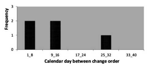
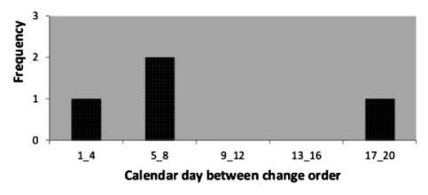
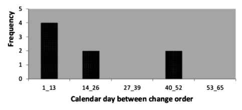
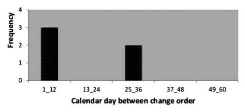
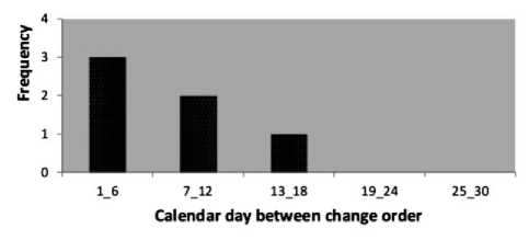
a) Time intervals between arrivals of events P01

b) Time intervals between the arrivals of events P02

c) Time intervals between the arrivals of events P03

d) Time intervals between the arrivals of events P04

e) Time intervals between the arrivals of events P05

Fig.2. Time intervals between arrivalsof events fordifferent projects.

• A.    Data from project deployments

The dataset used in this paper were obtained from a telecommunicationoperator in Ngaoundere. It comprises the data fromfive projects deployed in the Cameroon’s Adamawa region.

The dataset is structured as follows: the number of daysplanned for deployment, the initial cost of the project, thenumber of unexpected events that happened during deployment,and total cost of those events. Table 2 presents this datafor different projects.

Table 2. Deployments data

Project code	Locality	Initial period (days)	Initial cost (XAF)	Number of events	Unexpected cost (XAF)
P01	Nyambaka	30	11839859 0	5	2696310
P02	Mbe	12	11142340 9	4	1245079
P03	Doualayel	50	12344309 0	8	4338100
P04	Wack	36	11884159 0	5	12367400
P05	Dibi	20	11734709 0	6	1582800

The most convenient way to use the model proposed inthis study is to provide graphics or tabular solutions of theequations (18) and (26) which respectively give the probabilitythat the total cost of unexpected events remains below a certainpercentage of expected cost depending on contingencies. AMATLAB routine was designed [3] and the results are presentedbelow.

• B.    Statistical Analysis

We assumed that unexpected events occur after the Poissonprocess, which means that the time between the arrivals ofevents follows an exponential distribution. Histograms of time between events (figure 2) were plotted and the paces justifythis statement for all deployment projects studied.

Table 3.Rate of event per day

Project code	Original time (T)	Numberof Events(N)	Averagerate of event perday (α)	Expected number of events
P01	30	5	0.17	7
P02	12	4	0.33	3
P03	50	8	0.16	11
P04	36	5	0.14	8
P05	20	6	0.3	4

A closer look at figure 2 shows that in 80 % (4 of 5projects), histograms give the appearance of an exponentialdistribution. However, the project P02 rather gives the appearanceof a normal distribution or Poisson distribution that canbe approximated by a normal distribution. This justifies theuse of the Poisson process to find the number of unexpectedevents.

• C.    Probability of not having cost overrun

Table 3 provides the deployment parameters that havebeen considered: the total cost of unexpected events as apercentage of the original cost of the deployment project                       ∗100 and the rate of

\ initial cost/ events that happen per day.

In Table 3,

Number of eventsN

==

Number of daysT

The mean of these different rates give the following average rate:

a

m

У⁵ a

*-^ i = 1    i

= 0.22

Consideration has been made for testing: the average rate of arrival of the events was 0.22 events per day. For various contingencies in the original cost (1 %, 2 %, 5 %, 15 %, 20 %, 25 %, 30 %) and using the formula (18) of the proposed model, the probability that the total cost of unexpected events of each set of events is less than the above contingencies were obtained. We calculated the average of the probabilities to provide the results in table 4.

Table 4. Probability of not having cost overrun

Project code	X	( )
		e=1%	2%	5%	15%	20%	25%
P01	7	0.19	0.26	0.42	0.59	0.60	0.60
P02	3	0.32	0.40	0.53	0.58	0.59	0.59
P03	11	0.15	0.21	0.32	0.56	0.57	0.60
P04	8	0.17	0.23	0.39	0.58	0.59	0.59
P05	4	0.28	0.38	0.52	0.60	0.61	0.61

Finally, to see the effect of changes in contingencies on the probability of the cost of unexpected events, contingencies values were ranked, and the results are

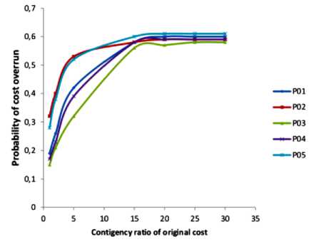
Fig.3. The probability of not having a cost overrun.

provided in Figure 3. This figure is equivalent to the graphical solution of the equation (18). This figure shows that the estimator can choose their contingency rates according to these means and the risk.

Most of the projects require a contingency of about 15%of the original cost to cover unexpected events.

• D.    Expected cost overrun

A Matlab routine implementing the formula (26) was used in order to determine the expected cost of contingency for different projects. To simplify the task, the average rate of arrival of events per day has been considered as the mean of the average rate of all deployment projects previously described. Using this mean rate and the time of deployment of the project, the expected number of unexpected events was obtained for each project. Through this, the total cost of the events of each set of events has been computed, and the average of these costs represents in this model the expected total cost of unexpected events. The result is presented in table 5.

Table 5. Expected cost of unexpected events

Project code	Cost overrun (XAF)	Cost overrun as ratio of original (%)	Expected cost overrun (XAF)	Expected cost overrun as ratio of original (%)
P01	2696310	2.28	3911957.95	3.30
P02	1245079	1.18	1665753.40	1.49
P03	4338100	3.51	6207674.17	5.02
P04	12367400	10.41	4637726.66	3.90
P05	1582800	1.35	2227404.54	1.89

The actual costs and expected costs of unexpected events of the various projects are shown in figure 4. In this figure, we find that four of the five deployment projects have an expected cost higher than the actual cost of contingencies; and one project has an expected cost lower than the actual cost. The big difference between the estimated value of the cost overrun of P04 and the actual value is due to the fact that unexpected events which occurred during the deployment of this project had very high costs; since in this model, we have for the total cost of unexpected events, the average costs of different sets as previously said. To overcome this problem, the cost of the set with the highest cost may be regarded as being the one desired. The main point is the fact that 80 % of expected cost are above and close to reality. From this, we can say that this model estimates realistically the cost of contingencies.

Fig.4. Real and expected costs of unexpected events.

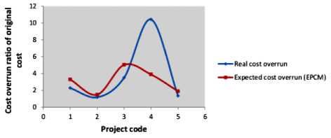
Figure5 compares the estimated costs using the PCM model, the proposed model and the actual costs of contingencies. In this figure, when observing the estimated costs with PCM model, two out of five projects have a lower cost to the reality; with the proposed model only one project presents this limitation. If we look on the model whose costs are close to reality, we find that both models (PCM and EPCM) provide realistic results.

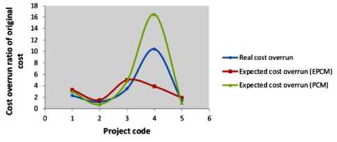
Fig.5. Real and expected cost (PCM and PCMM) of unexpectedevents.

• V.    Conclusion and Outlook

Information about unexpected events and data on past projects have been collected from telecommunications companies in the city of Ngaoundere, with the aim to develop a model that could fill gaps in the PCM model which is used to estimate the cost of a network deployment. The Poisson process was used to predict the number of unexpected events that may occur during network deployment. We obtained a model that provides results which are 80 % realistic according to the tests performed on the dataset. This shows the validity of this model. In fact, four projects out of five have a cost of unexpected events above and close to the original costs and needs contingency of 15% of the original cost to cover cost overrun. We can, therefore, say that our model is able to estimate reasonably the cost of unexpected events that may occur during deployment of a wireless network.

We intend to extend this model to be able to estimate the cost for deployment of wireless networks in urban areas by observing the unexpected events that often occur in these areas.