Extracting Feature Curves on Point Sets

Published Online June 2011 in MECS

Multiple techniques have investigated the identification of feature curves on point set models and polygonal models. The previous work on feature lines extraction can be roughly divided into three categories:

normal deviation based, covariance analysis based, projection procedure based.

Normal deviation based method proposed in paper [1] first estimates the normal vectors by the PCA analysis of these 1-ring neighbors, as explained in [2], and then the segmentation is performed on point cloud based on the variation of the normals. Once the connected graph where each edge connects two segments is constructed, the feature curves can be obtained after pruning and smoothing the graph.

Covariance analysis based methods [3] [4] classify the points of point cloud according to the likelihood or unlikelihood that they belong to a feature, which is computed from principal component analysis on local neighborhoods. In paper [3], by changing the local neighbor size, multi-scale estimation is achieved. Both [3] and [4] build minimal spanning trees over the potential feature points, and then curve lines are computed to appropriate the features. However, the above methods require high quality of point cloud, and their sensitivity to the smooth features is very limited.

Projection procedure based algorithm estimates the feature curves by approximating the point set surface. In paper [5], a robust algorithm that identifies sharp features in a point cloud by returning a set of smooth curves aligned along the edges. This feature extraction is a multi-step refinement method that leverages the concept of Robust Moving Least Squares (RMLS) [6] to locally fit surfaces to potential features. By projecting the points to the intersections of multiple surfaces, polylines are expanded along the projected points. After resolving gaps, connecting corners, and relaxing the results, the algorithm returns a set of complete and smooth curves that define the features. Since the RMLS is computationally expensive, this algorithm is limited by time constraints.

In this paper, we focus on extracting of valley-ridge lines from scatted point sets. The proposed algorithm falls into the third category of feature extraction algorithms, since it’s based on a projection procedure for local fitting. After approximating the neighborhoods of each point with a local MLS polynomial [7], the curvatures and curvature tensors are computed based on the first and second fundamental forms [8][9] of the surface. Points whose absolute value of principal curvatures is bigger than a threshold are defined as a potential feature point. By performing principal component analysis over the potential feature points, they are smoothed. Then feature curves are achieved by growing along the principal directions of the smoothed points.

The point clouds used in our experiments may contain connection information in originals, we only use their coordinate information.

Given an unorganized point cloud without normal and any connectivity information

P = { p } P i e R 3 , i e {1,..., N }, the valley-ridge curves on point cloud are achieved by performing the following four steps, see Figure 1.

• (1)    Approximating the neighborhoods of each point with a local polynomial, the principal curvatures of each point can be computed. Then the potential feature points are extracted according to the curvature values of each point.

• (2)    Based on Fundamental forms of fitting surface, the principal directions for each potential point are computed.

• (3)    Using cross-correlation coefficient analysis of local points and principal component analysis, we smooth the projected points.

• (4)    Create initial sets of valleys and ridges by growing polylines along the principal directions of the smoothed points, and then analyze the end-points of feature polylines to complete gaps.

In the following sections, we’ll discuss each of the four steps of the algorithm, in details.

• II.    P otential V alley - ridge points extraction

• A.    MLS fitting

The proposed algorithm employs moving least square (MLS) method to fit a smooth patch for to radius neighborhood of each point,

NBHD ( P i ) = ^{ P j ^}, \\ P j - рД\ < ю , j = 0,..., k , which works as follows.

Build a covariance matrix B of NBHD ( p_i ),

B = E    ⁽ P j - o i ⁾⁽ P j - o) T ■

P j e NBDH ( P i )

where

k

⁰ = /; E j = 1 ^Pj ■

Calculating the eigenvalues and their corresponding eigenvectors of B , a reference domain H_i is defined by eigenvectors which are corresponding to the biggest eigenvalue and the second biggest eigenvalue, respectively. The surface normal n_i of H_i is set to be the eigenvector corresponding to the smallest eigenvalue, \\ n i \\ = 1. Then build a local coordinate system on H i , o i is the origin and n_i is the Z -axis.

(a)

(b)

(c)

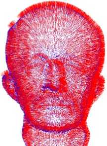
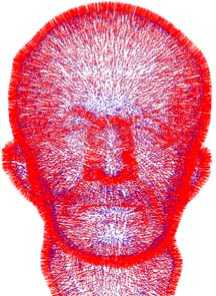
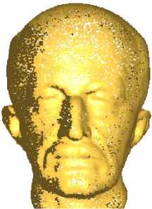
Figure 2. Normals of Maxplanck model before adjustment and after adjustment. (a) Normals before adjustment (b) Normals after adjustment (c) point cloud with unadjusted normals (d) points set with adjusted normals.

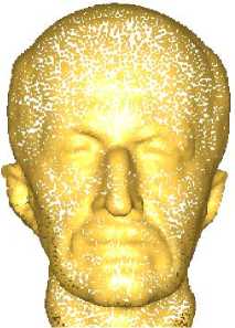
(d)

The experiment shows that the Z -axes of local coordinate frames can point to the different sides of point set ‘surface’, see Figure 2(a). For the purpose of obtaining right valley-ridge information, consistently outward normal directions are adjusted by applying normal adjustment operation [10]. And each + Z axis of local coordinate system has the same direction as the adjusted n_i , see Figure 2(b). Then NBHD ( p_i ) is approximated with a local MLS polynomial g_i which satisfies (1).

min E < Pj - Pg, n >2        (1)

P j e NBHD ( P i )

p_g is the projection of p_j onto g_i along n_i . g_i is a polynomial in local coordinate ( o_i , u , v , n_i ) , i.e.

g_i ( u , v ) = a + bu + cv + duv + eu ² + fv ²,( u , v ) ∈ [ - h , h ]²

Formula (1) can be changed to

min ∑    ((pj-oi)⋅ni-g(uj,vj))2     (3)

p_j ∈ NBHD ( p_i )

here, ( u _j , v _j ) is the representation of p_j about a local coordinate system in H_i . For any point q in H_i , its projection on g_i can be calculated out as o_i + ( u_q , v_q , g ( u_q , v_q )).

Since the resulted MLS approximation relies on the number of neighbor points used in local fitting, we set the fitting radius to = 2.0* К , where К denote the average station distance of the point cloud.

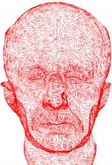
determined, as shown in Figure 4. Since T _max and T _min are everywhere orthogonal (expecting for umbilical region), it only needs to compute one of the curvature direction fields, and the other direction field can be achieved by computing its gradient field.

In our feature curve extraction process, to speed up the whole procedure, only principal directions of detected potential feature points are calculated, as seen in Figure 1(c).

(a)

(b)

(c)

(a)

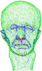
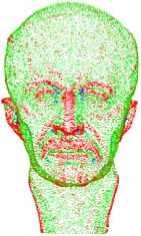
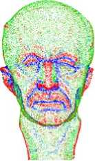
Figure 4. Principal directions T max , T min estimated on point set surface. (a) Maximal principal directions. (b) Minimal principal directions.

(b)

Figure 3. Point set marked according to the value of principal curvatures. (a) Maximal principal curvatures. (b) Minimal principal curvatures. (c) The biggish principal curvature values.

IV. S moothing the feature points

• B.    Curvatures computation

Since the local fitting g_i has been achieved, curvatures of each point p_i on point set surface can be calculated based on computing the first and second fundamental quality of the surface [8] [9]: L, M, N, E, F, G. The main curvatures of p_i are denoted as K _max , K _min . Based on the analysis of the experiment results, we found that better results are achieved by using biggish principal curvature, see Figure 3.

• C.    Potential feature points detection

k_i is the biggish principal curvature of p_i , τ is a user defined threshold which related to the average absolute curvature of the whole point set. If k_i <  0 and | k_i | > τ , p_i is added into valley-point set V , if k_i >  τ , p_i is added into ridge-point set R , see Figure 1(b).

As a matter of convenience, we use F representing V or R in the following paper.

• III.    C omputing principal direction of minimum

CURVATURE

Based on the fundamental forms of fitting surface, the principal directions responding to K _max , K _min can also be calculated as follows:

T max = (( - 1)*( N - K max G ), M - K max F )

T min = (( - 1)*( N - K min G ), M - K min F ),

By computing the principal directions of each point in point set, curvature tensor on point set surface can be

The feature points are smoothed by projecting them onto their principal axis of neighborhoods, so the over all smoothing performance is determined by the neighborhood size δ , as seen in Figure 5. In order to obtain stable smoothing effect, adaptive neighborhood growth scheme, which based on a statistical analysis of point distributions on the approximate plane, is adopted [5].

For each potential feature point p_i ∈ F , the covariance matrix C of the neighborhood

NBHD(pi)={pj|(||pj-pi||≤δ,j=0,...,k)} is computed,

C=(p1-p,...,pk-p)⋅(p1-p,...,pk-p)T where

1 k ^{p =} k ∑ j = 1 ^p

j .

Calculate the eigenvalues and their corresponding eigenvectors, let λ0≥λ1≥λ2, then V0 , V1 , V2 are corresponding eigenvectors of λ0,λ1,λ2. Project feature points onto the plane defined by two eigenvectors V0 , V1 and p . Then the projected points are translated into the local coordinate, and the projected points are interpreted in terms of a distribution of two random variables, X and Y , which can be analyzed by crosscorrelation coefficient defined by

₌ cov( X , Y )

^{ρ XY =} D ( X ) D ( Y )

where, ρ _XY has value between -1 and +1 representing the degree of linear dependence between X and Y , meaning that the points in NBHD ( p_i ) are distributed along a feature line.

δ will be increased if the cross-correlation coefficient ρ over points in δ neighborhood is not sufficiently large enough, for our models we use ρ ≥ 0.6 . i f δ is bigger than a predefined threshold, the point p_i will be abandoned as outlier or noise.

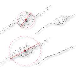
Figure 5. Smoothing result in different neighborhood size [5] [11].

After getting a suitable δ , the principle axis of new NBHD ( p_i ) is obtained by employing PCA operation, and then a smoothed point p & _i is yielded by projecting p_i onto the principle axis.

The smoothed points are added into the point set of F ( S ) .

• V. F eature polyline propagation

Feature polylines of valleys or ridges are respectively generated by growing them along the maximal principal curvature directions of V ( S ) and minimal principal curvature directions of R ( S ).

• A.    Growing of a feature curve

For a new line of feature curve, seed point is traced in each principal direction D as:

D ∈ { T max , - T max } or { T min , - T min }

Suppose L = { l ₁ , , l_n } be the current generating curve, where l_k is the k-th sample point. The new point on current curve is generated as:

lk=lk-1+s⋅dk-1

where s indicates a user-specified step size, and d_{k - 1} is the principal direction of l_{k - 1} . Since l_k probably not exactly belongs to the point set surface, it needs to be optimized. The neighbor points in radius r are collected and the barycenter p_c is computed. Arranging the concerned principal directions of neighbor points as the same sign with the direction vector of l_{k - 1} , the principal direction of p_c is computed as the unity vector of the neighbor’s, which normalized and denoted as T_c . Then l_k is set to be the barycenter p_c and its principal directions is set to be T_c .

Once the new updated sampled point is obtained, the neighbors of the previous sampled point in radius s are tagged and will not be concerned in the following tracing operation. However, for the starting seed point, not all its neighbors in radius are tagged, but only the points in the semi-sphere of the current tracing direction, as shown in Figure. 6.

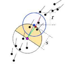
(a)

Figure 6. The lines of curvature tracing process. The Purple point is the starting seed, the blue point is the new sampled point, and the red point is the optimized new sampled point. When a new sampled point is detected, the neighborhoods of the previous sampled point are flagged. (a) The tracing process in one direction of the seed point. (b) The tracing process in the other direction of the seed point.

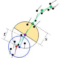
(b)

Each current feature curve stops, if any one of the following conditions is satisfied:

• (1)    If the neighbors of current sampled point in radius r has been tagged.

• (2)    If a feature line reaches the boundary of the point set, i.e., there are no neighbors of the current sampled point in radius r .

The two parameters ( s and r ) used in the tracing process are both related to the average station distance of the points cloud κ . Our experiments indicate that s = 1.2 * κ and r = 0.8 * κ lead to good results.

• B.    Lines of valleys and ridges extracton

The feature curves of valleys and ridges are extracted independently. And the sampled points of feature curves are separately added into the point set R ( L )and V ( L ). Since the ridges and valleys turn into each other as surface orientation is changed, without loss of generality, only the lines of ridge curves are considered, which are extracted by performing the following steps:

• (1)    All points in R ( S ) are added into a priority queue, the points with higher ratio between maximal principal curvature and minimal principal curvature are assigned higher priority.

• (2)    Pop a new seed point p_i from the priority queue and add it into R ( L ) as l ₀ . Then a tracing procedure is separately started from l ₀ in two different directions T _min , ^- T min .

• (3)    During the tracing process, for each new sampled point l_{k + 1} , if none of the stopping conditions are satisfied, the new sampled point l_{k + 1} is added into R ( L ). And then the local neighbors of the previous sampled point l_k in radius s are flagged and removed from the priority queue. Otherwise, the tracing operator of the current direction needs to be stopped.

By repeating steps (2) and (3) until the priority queue is empty, the feature curves of ridges are obtained, as shown in Figure 1(f).

The feature curves of valleys can be calculated based on the same scheme as tracing feature curves of ridges.

• C.    Optimization of Feature Curves

Then gaps between polylines which are caused by poor sample quality are completed by connecting each endpoint of feature polyline to other feature points within the cone formed by the tangent vector T at the end-point and a predefined aperture angle µ [5].

Finally, we smooth polylines by applying uniformity scheme on interior points for 1 or 2 passes. Given a feature polyline R = { q ₀,..., q_k } , firstly fix q ₀ and q ₂ , then do the following work on the plane which defined by ( q ₀, q ₁, q ₂) : move q ₁ to the vertical of the line segment ( q ₀, q ₂) with no change of the area of triangle Δ q ₀, q ₁, q ₂ . Repeat this until all internal vertices are adjusted, see Figure 7.

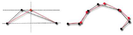
Figure 7. Smoothing feature polylines; fix the end-points of the polylines and adjust the internal vertices with restriction that the area of any triangle enclosed by three contiguous points keeping invariant on their own defined plane.

As seen in Figure 8, the valley and ridge feature curves are extracted from Sper-dragon models.

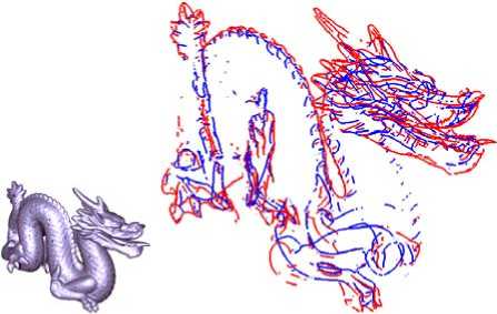
Figure 8. Valley-ridge feature curves on Sper-dragon model, blue lines denote valleys and red lines denote ridge curves.

The performance of the proposed method to its run time efficiency and robustness to noise is discussed in this section. The proposed algorithm carried out on a 2.7GHz AMD Athlon 2.7GHz processor with 2GB memory.

• A.    Run Time Efficiency

Since the experimental data used in our algorithm are raw point clouds without any normals and connection information, the preprocessing operators including normal computation and orientation arrangements are essential parts of the feature curve extraction. The moving least squares surface fitting is a fundamental operation for detecting potential feature points and computing principal directions of each feature points. Smoothing potential feature points and generating feature curves are the last two key procedures for the proposed algorithm.

As shown in Table I, we technically divide the whole running time of the algorithm into four parts: (1) cost for pre-processing including normal calculation and average station distance. (2) Cost for MLS fitting, curvature estimation, and also includes the cost of detecting potential feature points. (3) Smoothing feature points, and feature curve propagation and completion. The experiments indicate that the most time-consuming part of our implementation is the preprocessing (1) and MLS surface fitting (2). Since the time required to construct the polylines of feature curves is determined by the number of potential feature points in point cloud, the cost of (3) increase when models have complicated details.

• B.    Robustness to Noise

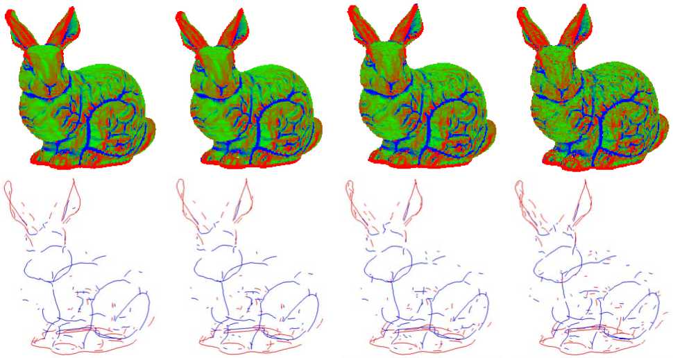
  To validate the robustness of the extraction of feature curve in handing noisy point sets, three sets of noisy data are generated by adding Gaussian noise with different amplitudes of standard deviations (i.e. 0.0001 and 0.001) to each point cloud model. Table II shows that an increase in the noise level leads to a slight increase in the computational costs, which can be explained by the fact that, for models with higher noise level, the same curvature threshold and MLS radius leads more potential feature points, which consequently increase the cost of (3). The graphic illustrations in Figure 9 also indicate that the proposed algorithm is very stable against noise.

• VI. E xperiments R esults

TABLE I.

T HE RUN TIME PERFORMANCE OF THE PROPOSED ALGORITHM WHICH COMPUTED WITH ω = 2.0 κ , τ = 16 . [ κ = A VERAGE STATION DISTANCE , ω = MLS RADIUS , τ = CURVATURE THRESHOLD FOR DETECTING FEATURE POINTS ]

Model	Scale [Point]	κ [10-2]	Feature Points	Run time (ms)
				(1)	(2)	(3)	Total
Maxplanck	25445	1.6130	5771	1046	625	204	1875
Bunny	35947	1.7479	4434	1437	860	156	2453
Venus	134359	0.9094	25215	5141	3359	1688	10188
Balljoint	137073	0.6924	46911	1985	3718	4954	10657

TABLE II.

T he run time performance of the proposed algorithm performing on different models at varying noise levels with to = 2.0 к , T = 16 . [ К = A verage station distance , to = MLS radius , T = curvature threshold for detecting feature points ]

Model	Scale [Point]	Noise	К [10-2]	to [ К ]	T	Feature Points	Run time (ms)
							(1)	(2)	(3)	Total
Maxplanck	25445	0.0001	1.6134	2.0	16	5803	1047	625	234	1906
		0.0005	1.6131	2.0	16	5972	1047	625	235	1907
		0.001	1.6113	2.0	16	6597	1047	609	281	1937
Bunny	35947	0.0001	1.7468	2.0	16	4452	1438	859	141	2438
		0.0005	1.7455	2.0	16	4508	1438	859	141	2438
		0.001	1.7426	2.0	16	4802	1438	859	172	2469
Venus	134359	0.0001	0.9090	2.0	16	25274	5094	3359	1641	10094
		0.0005	0.9094	2.0	16	30153	5125	3344	2359	10828
		0.001	0.9063	2.0	16	30153	5125	3328	2407	10860

• (a)                           (b)                            (c)                             (d)

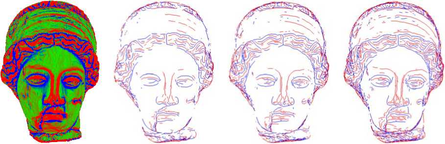
Figure 10. Multi-level valley-ridges curves extraction on Venus models, where blue lines indicate valleys and red lines indicated ridges. (a) Venus model colored according to the biggish principal curvatures. (b) Features computed with curvature threshold T = 16 . (c) T = 13 . (d) T = 10 .

(a) 0.0

(b) 0.0001

(c) 0.0005

(d) 0.001

Figure 9. The feature curves extracted on bunny models witch is added with different level of Gaussian noise. Blue lines denote valleys and red lines denote ridges. The bunny models with different noise are color marked according to the biggish principal curvatures on the top line. The feature curves are respectively depicted on the bottom line. (a) Models with no noise. (b) Models with Gaussian noise of 0.0001. (c) Models with Gaussian noise of 0.0005. (d) Models with Gaussian noise of 0.001.

• C. Multi-resolution Extraction and Error analysis

Multi-resolution valley-ridge features are achieved by applying different radius in local surface fitting, and using different curvature threshold in valley-ridge point detection. As seen in Figure 10, multi-resolution feature curves are achieved on Venus models computed with to = 2.0 k and with varying curvature threshold of t = 16 , T = 13 , t = 10 .

The valley-ridge feature points extracted by our algorithm may not be the points in point set, but the points projected onto the local MLS fit, so the error of our implication is the error of MLS surface fitting [12].

• VII. C onclution and F uture W orks

This paper present a new algorithm for extracting valley-ridge curves from raw point cloud, the experiments indicate that the proposed algorithm produces viable results on irregular point clouds (see Figure 1) and point data with different level of noise(see Figure 8, 9) in high efficiency, and meanwhile, the multiresolution feature curve can also be achieved (see Figure 10).

As future work, we plan on improving the computing efficiency of detecting potential feature points, and investigating the smoothing and sampling methods to preserve both sharp features and smooth features.

A cknowledgment

The work in this paper was supported by National Natural Science Foundation of China (Grant No. 61002040 and Grant No. 60873175).