Fast and Accurate Classification F and NF EEG by Using SODP and EWT

Published Online November 2019 in MECS

Detection of brain disorders using Electroencephalogram (EEG) as a nonstationary signal is one of the oldest challenge in biomedical signal processing applications. Epilepsy is a neurological disorder due to abnormal conflict for human brain whereas focal (F) epilepsy happens in the limited area of brain [1]. In contrast to F signal, the nonfocal (NF) refers to the normal EEG signals. Removing the brain part, which is the epilepsy source attack, is a surgery solution for these drug resistant patients. So, the epilepsy localization area is an essential step before surgery. The areas belonging to F signal can be identified by visual inspection of EEG signals, which is boring and timeconsuming being prone to errors. Therefore, distinguishing the F and NF EEG signals may help detecting the abnormal part of an epileptic patient’s brain. So, in recent years, researchers have proposed methods [1-8, 11] in order to classify the F and NF EEG signals.

In [1], F and NF EEG signals were distinguished based on delayed permutation entropy and support vector machine (SVM). In [2,3,4], empirical mode decomposition (EMD) was applied to decompose the EEG signals into their intrinsic mode functions (IMFs). In order to discriminate between F and NF signal, entropy based features extracted from IMFs were applied for least square SVM (LS-SVM) in [2], nonlinear features extracted from IMFs were applied for SVM in [3], and log energy entropy was computed in EMD-DWT (EMD-Discrete Wavelet Transform) domain in [4]. Detection of F EEG signals using features derived from Fourier-based rhythms was proposed in [5], and various features of entropies derived from DWT coefficients were used in [6]. In [7], fractal dimension of flexible analytic wavelet transform coefficients have been extracted as features and fed to robust energy based least square twin SVM (RELS-TSVM). Recently, autoregressive model and entropy based features have been computed in variation mode decomposition (VMD)-DWT domain for classification of F and NF EEG signals [8].

Although most of methods have been based on entropy features, 2D projection of EEG signal rhythms were plotted by using the reconstructed phase space (RPS) in empirical wavelet transform (EWT) domain for the first time [9]; they computed average logarithmic areas from 2D RPS of rhythms as features. In other words, they used degree of variability for EEG rhythms to distinguish F and NF signals. The results of the proposed method [9] was promising, though, it was time-consuming. In [9], the EEG signal was first separated to delta (δ), theta (θ), alpha (α), beta (β) and gamma (γ) rhythms using EWT. Then, 2D projection of rhythms was plotted, the areas were computed as features, and finally the LS-SVM classified the signal. In comparison with the other parts of the algorithm, the RPS block was time-consuming. This is because RPS matrix needs optimum values of delay time τ and embedding dimension d, which is computed from the input signal by mutual information [10,11] and false nearest neighbor methods [10]. In [12], the influence of differential features were investigated in F and NF EEG signals classification indicating that differential features can play better performance in F signal detection. The second order difference plot (SODP) is a graphical representation of successive rates against each other and provides the data variability rate [13]. SODP can represent the different EEG signals in 2D space faster than RPS because it does not require computing any parameter.

In this paper, SODP is used instead of 2D RPS in order to speed up the algorithm run time, and also classify F and NF EEG signals accurately. For this purpose, EEG signals are decomposed to their rhythms in EWT domain. The motivation of working on EEG rhythms comes from the success of using rhythms in previous studies [5,9]. After that, SODP of each rhythms is projected and then radius (r) of various central tendency matures (CTMs) are determined and put into ln( n r 2 ) as features. Kruskal-Wallis statistical test is applied to obtain significant features, which are fed into SVM and k nearest neighbor (KNN) classifier with various kernels and distances, respectively.

The paper is organized as follows. Section II reviews DWT and EWT. In Section III, the proposed method for F and NF discriminating is presented, which consists of rhythm separation, SODP, and feature extraction. Section IV presents the experimental results and discussion. Finally, the paper ends up with a conclusion in Section V.

• II.    A Review Of Dwt And Ewt

In general, DWT uses filter bank to decompose a signal into specified frequency sub-bands. The cut-off frequency ( f ) of the filter bank at the first and the second decomposition levels are я/2 and П4 in order, so it is я/2n at the n-th decomposition level. In other words, for the n-th decomposition level, the low-pass and high pass band-width filter are [0, П2n ] and[ n]2n , я/2n+1 ], respectively. Two functions, called Ф as scaling function, and Ψ as wavelet function, have key roles in signal decomposition. Accordingly, different wavelets such as Haar [13], Daubechies (db) [15], and Symlet [16] have been proposed so far. For every decomposition level, the signal projection with low-pass filter and high-pass filter are called approximation and detail, respectively. However, the f in DWT for all decomposition levels is constant meaning that the DWT is not adaptive according to the input signal [17].

EMD has been proposed to decompose nonlinear and nonstationary signals into IMFs. Sensitivity to noise and sampling frequency, lack of mathematical theory, and mode-mixing are important drawbacks of the EMD method [17].

EWT is proposed to compensate the non-adaptive of DWT and EMD defects [17]. The EWT extracts different modes of a signal by building adaptive wavelets. In contrast to DWT, bandwidths of the EWT filter bank are not constant and vary according to the input signal components. In [17], the number of modes (L) is assumed to be fixed. Using Fourier transform, the frequency spectrum of the input signal is obtained in [0, я ]. Also, the L-1 local maxima of frequency spectrum are marked, and then midpoints of every pair maximum are used as the bandwidth of EWT filter bank, which enables EWT filter banks to be adaptive. After specifying segmentation of spectrum and determining bandwidth of filter bank, the filter bank is formed according to the idea of Littlewood–Paley and Meyers wavelets [18]. For EWT, the scaling function and the wavelet function are defined in Fourier domain as [17],

^ ( ® ) = * cos(-

лР(2, ® 1 )

)

( ® _z ) = -

cos(

• пв ( 2 , ® _{+ 1})

sin(

™p^{( 2 ,} ® f ) .

)

if |® / | < (1 — 2 ) ® 1 if (1 - 2 ) ® <  ® |< (1 + 2 ) ® otherwise

,f (1 + 2 ) ® , < ® <  (1 - 2 ) ® , _{+ 1} ,f (1 - 2 ) ® , _{+ 1} <  ® f | <  (1 + 2 ) ® , ₊ i f (1 - 2 ) ® , <  ® _f | <  (1 + 2 ) ® ,

otherw se

.                     ®, -(1-2), where p(2, ®) = e(^-f-------) , and ® is the band-

‘22® width       of       EWT       filterbank,

®,=1,2^ m ={[0, fCMS],[ fcuv fu2],...,[ f™.,- -1, П]} and в ( У ) is, ffУ

в ( 2 ) = * в ( У ) + в (1 - У ) = 1 f   V У Е [0,1]

ifУ and

.       .    .®i + 1    ®i.

2 <  min (---------)

®i+1 + ®i which make sure, the EWT coefficient are in L (^) space. Also, 2 parameter tightens up the filter bank frame and causes that bandwidths have the lowest overlapping with upper and lower frequencies. Furthermore, 2 parameter makes EWT filter bank to have ignorable stop-band ripples. In other words, 2 is able to solve the mode-mixing problem. Similar to DWT, signal projections with scaling and wavelet functions are called approximation and detail coefficients, respectively.

• III.    Proposed Method

In this paper, EEG signals are separated to rhythms by using EWT. Then, SODPs of each rhythm are plotted, and the value of ln( n r ²) corresponding to every CTM is considered as feature ( r is the circle radius). Finally, extracted features are fed into KNN and SVM classifiers to distinguish F and NF EEG signals.

Bern Barcelona EEG database [19], including 50 pairs of F and 50 pairs of NF EEG signals, is used in this paper. Each pair has two columns, named “X” and “Y”, recorded from adjacent channels. All EEG signals have 10240 samples, and the duration of every signal is 20 second, so sampling frequency is 512 Hz. The EEG signals belong to five epilepsy patients who were candidates for the brain surgery. In this work, 50 pairs EEG signals from F and NF groups are chosen to evaluate the proposed method [1-7,9]. Fig.1. shows samples of “X” and “Y” channels, EEG signals, and “X-Y” for F and NF groups. According to our experimental results, for considering “X-Y” as the input, the NF EEG signal in comparison with F EEG signal has more energy and less standard deviation.

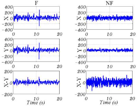
Fig.1. From up to down are “X’’, “Y” and “X-Y” of F (left) and NF (right) EEG signals. As seen in last row, the amplitude of NF signal is greater than F for “X-Y”.

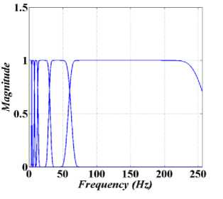
Fig.2. Shown the EWT filter bank for rhythm separation.

• A.    Rhythm Separation by DWT and EWT

In general, EWT was proposed to decompose nonstationary signals [17], and it has already been used for detecting Parkinson’s [20] and glaucoma [21]. EWT generates filter bank by proper segmentation of input signal spectrum. For signal spectrum segmentation, ‘local maxima’ [17], ‘histogram’ [22] and ‘scale space’ [23] have been used so far.

*********** ef fH«**»M *

NF i^frA^^VwVM^^

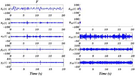
Fig.3. From up to down, shown the separated δ, θ, α, β and γ rhythms of “X-Y” for F (left) and NF (right) signals. The amplitude of NF signal for all five rhythms is greater than the F EEG signal.

In this paper, the spectrum of input signal in Fourier domain is segmented to extract the five EEG rhythms. The cut of frequencies of the filter bank set feut = {4,8,13,30,60} Hz, or the filter bank band pass are [0, 4], [4, 8], [8, 13], [13, 30], and [30, 60] corresponding to δ, θ, α, β and γ rhythms. Experimentally, the value of 2 in EWT (see Section 2) are set 0.2381 to avoid the overlapping of sub-bands. As EWT filter bank generates tight frame, transition bands of the filters are small, and pass-band and stop-band ripples are negligible [17]. As a result, pretty less aliasing occurs through rhythms separation mean3ing that EWT is able to separate rhythms precisely. Fig.2. shows the generated filter bank to separate EEG rhythms, where the first five filters separate δ, θ, α, β and γ rhythms. It should be noticed that frequency content greater than 60 Hz are considered as noise. Fig.3. shows the extracted five rhythms for EEG signals of F and NF samples. As seen in Fig.3. and it was expected according the results shown in Fig.1., for all five rhythms, the NF EEG signal has greater energy and standard deviation (std) in comparison with F EEG signal.

Although many researchers, e.g. [3,5,23] used DWT for extracting the five EEG rhythms, in this paper (see Section 2), a signal is decomposed into six levels by DWT, with one approximation and six details. Obviously, details 1, 2 with frequency bands [128, 256] and [64, 128]

Hz are noise and should be ignored. Details 3, 4, 5, and 6 with frequency bands [32, 64], [16, 32], [8, 16], and [4, 8] in order are considered as γ, β, α, and θ respectively. Finally, approximation with the frequency band [0, 4] Hz is δ as well.

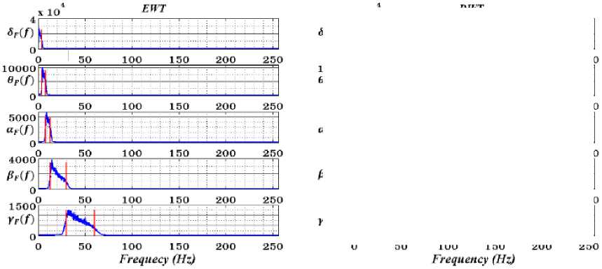
Fig.4. Shown the average spectrum of extracted separated δ, θ, α, β and γ rhythms (first-fifth rows) of ‘X-Y’ by using EWT (first column) and DWT (second column) for EEG signals.

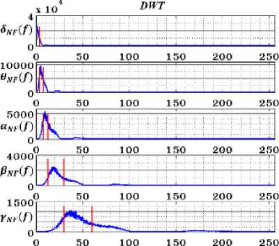
DWT and EWT are decomposed using db4, and the spectra of extracted rhythms on average are shown in Fig.4. Accordingly, frequency leakage for all DWT outputs is the main drawback because of exiting stopband ripple in comparison with EWT without considerable leakage.

• B.    SODP for 2D Projection of Rhythms

As explained before, SODP [13] represents the variability of a signal x (n) by plotting Y (n) versus X (n):

X ( n ) = x ( n + 1) - x ( n )             (4)

Y ( n) = x ( n + 2) - x ( n + 1)           (5)

Actually, SODP shows the differences of input signal x (n) in 2D projection. Recently, SODP was used for human identification [25] in electrocardiography (ECG) signal, seizure epilepsy [13] in EEG signal, and chronic obstructive pulmonary disease [26] in lung sound signal. Fig.6. shows the SODP of rhythms of a sample F and NF EEG signal.

• C.    CTM for Feature Extraction

CTM measures the degree of variability in 2D plot [27], i.e. SODP in here. Supposing that all data points in 2D projection are N and a circle with radius r covers M data points, CTM is defined as the ratio of M/N,

1 ^N

CTM =   £ q ( b n )                   ⁽⁶⁾

N n = 1

Г 1 if   ([ X ( n )]² + [ Y ( n )]²)^1/2 <  r

^{q (} b n )=L                     .

1 0                otherwise

For all five rhythms, the CTMs for different r (s) are computed, and then the corresponding value of ln( n r ²) is considered as feature.

• IV.    Experimental Results And Discussion

Each file in Bern Barcelona database consists of two EEG signals; i.e. “X” and “Y” as shown in Fig.1. According to [3, 4] the difference value of “X-Y” is recommended as input. The motivation to analyze the signal “X-Y”, i.e. the difference between two adjacent channels, comes from its robustness to noise and interference reported in various algorithms related to F

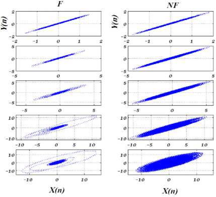
Fig.5. Shown the SODP of δ (first row), θ (second row), α (third row), β (fourth row) and γ (fifth row) rhythms of ‘X-Y’ of F (first column) and NF (second column) EEG signals.

signal detection. EWT segments the five EEG rhythms of δ, θ, α, β and γ of input signal “X-Y” as shown in Fig.3.

The SODP is then obtained for every rhythm. As shown in Fig.5. the SODP of F for all rhythms has more regular geometrical shape in comparison with NF EEG signal. Also, it is expected that the std of F to be less than NF for all rhythms. In this paper, CTMs is used for M/N= 20, 40, 60, and 80% (see Eqs. 6-7), followed by obtaining the corresponding r value and computing ln( π r ² ) as feature. So, the feature vector length is 5 (i.e. CTM ^δ M /_N,CTM_M/_N, CTM_M/_N,CTM_M/ N ,CTM ^γ M/ _N ).

As expected and also based on mean std and p-value of the extracted features (Table 1.), the std of F is less than NF for the all computed CTMs, and all EEG signal rhythms. Equivalently, as it was approved in [1], F signal has lower entropy in comparison with NF signal. Now, Kruskal–Wallis statistical test is used to obtain significant features according to their features with p-values of <0.05, which are then fed into the classifier.

Table 1. indicates that all rhythms, except ‘theta’, satisfy a p-value of < 0.05, so the feature vector size for every CTMs consists of four elements (i.e. CTM ^δ M / _N,CTM_M/_N, CTM_M / N , CTM ^γ M / _N ).

SVM [3, 4, 9] and KNN [4, 7] are two well-known classifiers. SVM maps the input data to high dimensional space to construct an optimum hyper plane by using different kernels such as radial basis function (RBF) and quadratic kernel functions (QKF).

Table 1. The results (mean, standard deviation (std) and p-value) of features extracted from rhythms of EEG signals.

Feature	Statistical parameter	δ	θ	α	β	γ
CTM	F(mean±std)	-1.76±1.36	-1.34±1.27	-1.43±1.43	-0.28±1.37	0.43±1.31
	NF(mean±std)	-2.59±1.59	-1.39±1.53	-0.81±1.59	0.57±1.69	1.39±1.75
	p-value	5.13×10-3	6.74×10-1	2.90×10-3	1.67×10-4	4.35×10-5
CTM40	F(mean±std)	-0.29±1.38	0.11±1.29	0.00±1.44	1.00±1.37	1.48±1.33
	NF(mean±std)	-1.14±1.58	0.05±1.53	0.61±1.59	1.82±1.68	2.37±1.75
	p-value	5.35×10-3	7.51×10-1	5.95×10-3	2.32×10-4	8.27×10-5
CTM60	F(mean±std)	0.67±1.39	1.10±1.32	1.02±1.46	1.96±1.38	2.33±1.34
	NF(mean±std)	-0.16±1.56	1.02±1.54	1.58±1.58	2.74±1.68	3.14±1.74
	p-value	7.95×10-3	8.20×10-1	1.36×10-2	3.56×10-4	1.67×10-4
CTM80	F(mean±std)	1.57±1.38	2.04±1.34	2.01±1.50	2.92±1.38	3.23±1.36
	NF(mean±std)	0.76±1.56	1.95±1.54	2.48±1.60	3.60±1.67	3.92±1.74
	p-value	1.05×10-2	7.88×10-1	3.37×10-2	1.41×10-3	6.77×10-4

Table 2. Performance of SVM classifiers using various kernel functions for extracted features.

SVM classifier	QKF kernel function				RBF kernel function
Features	CTM	CTM40	CTM60	CTM80	CTM	CTM40	CTM60	CTM80
ACC (%)	89	89	88	86	90	91	88	85
SEN (%)	90	94	90	90	94	94	92	88
SPE (%)	88	84	86	82	86	88	82	82
Kernel parameter	-	-	-	-	0.8	0.7	1.4	1.3

Table 3. Performance of KNN classifiers using various distances for extracted features.

KNN classifier	City block Distance				Euclidean Distance
Features	CTM	CTM40	CTM60	CTM80	CTM	CTM40	CTM60	CTM80
ACC (%)	92	93	90	88	91	92	90	86
SEN (%)	98	100	96	90	98	94	98	90
SPE (%)	86	86	84	86	84	90	82	82
Number of neighbors	4	4	4	2	4	2	4	9

In contrast, KNN maps an input test sample to a group with more members among its k nearest neighbors. Number of k and distance type are the two justified parameters in KNN. In this paper, we suppose k ∈ [2, 9] and use Euclidean and city block distances. In general, the classifier outputs are categorized in one of the four different cases listed below.

TP (true positive): the number of F EEG signals identified as F EEG signals.

TN (true negative): the number of NF EEG signals identified as NF EEG signals.

FP (false positive): the number of NF EEG signals identified as F EEG signals.

FN (false positive): the number of F EEG signals identified as NF EEG signals.

Accordingly, accuracy (ACC) measures the algorithm capability to discriminate F and NF signals, and sensitivity (SEN) and specificity (SPE) measure the algorithm ability to determine in order F and NF cases correctly [28].

TP+TN

ACC = -------------x 100

TP+TN+FP+FN

TP

SEN = ------X 100

TP+FN

TN

SPE =

TN+FP

In general, K-fold cross validation [29] is used to break the data into train and test to be used by the classifier. Actually, for k-fold cross validation, k time, k-1 subset are used to train, and one resume subset is used to test the classifier. Finally, mean value of objective parameters is reported. In this paper, ten-fold cross validation and the objective parameters are used as in Table 2. and 3. Accordingly, and also exactly the same as that reported in [9], CTM among four CTMs is recommended irrespective of the classifier type and its parameters. However, maximum ACC reported by [9] using 2D RPS rhythm for CTM was 90% where as ours is 93% showing the superiority of the proposed algorithm using 2D SODP rhythms and EWT. In addition, the algorithm run time for processing every EEG signal was 8 seconds in [9] while ours is only 0.08 second using Intel (R) core (TM) i5-M480 CPU (2.67 GHz), 6GB RAM, and MATLAB 2014a.

At the end of this section, the proposed algorithm using SVM and KNN classifiers is compared with state-of-the-art papers in term of three predefined objective criteria (ACC, SEN, SPE), where the feature vector lengths are also reported. All algorithms used 100 EEG signal from Bern Barcelona dataset [19]. The results, written in Table 4., clearly indicate that our proposed method achieved the highest classification ACC in comparison with other techniques. However, the feature vector length is less than other methods, except reference [9] with the same feature vector length.

• V.    Conclusion

Using EWT to extract the EEG rhythms, SODP to provide the data variability rate, and KNN and SVM to classify F and NF signals showed that the proposed method is outstanding in comparison with state-of-the-art-papers not only in terms of three objective criteria but also according to the feature vector length affecting the algorithm complexity. However, using few number of patients whose EEG signals were recorded, obtaining sigma value in SVM and number of K in KNN empirically are the bottlenecks that should be resolved in future works. In addition, it is recommended to measure the 2D space complexity as a parameter for classification.

According to our experiments, the proposed method is also recommended for processing the ECG and the electromyogram (EMG) signals in order to early detect cardiac and muscular diseases.

Table 4. Comparison between the proposed method and previous studies where the same database used.