Fast generation of image’s histogram using approximation technique for image processing algorithms

Published Online March 2018 in MECS

Image processing algorithms normally will take an image as input and generate image as output. The input image which is transformed by function(s) to generate the output is presented in a form of dataset with spatial arrangement of pixels. The transformation processes in both image processing and computer vision task are usually based on statistical operations [1] or involve a number of statistical subtasks. Most of these statistical subtasks are effectively performed when the histogram of the image is known. Information such as image’s mean, median, mode, variance, and standard deviation can easily be computed when the histogram of a given dataset is provided. The histogram is just an arrangement of bars, with the height of the bars representing the ratios of the various data values. The higher bars in a histogram represent more data values in a class, while lower bars represent fewer data values in a class and these classes have been explored extensively for analysis of the nature of a given dataset. The nature of the distribution in the histogram also enables algorithms to select values for further operations. The generation of Probability Density Function (PDF), Cumulative Density Function (CDF), Histogram Normalization, and Histogram Equalization (HE) which are widely used in image processing and computer vision task can easily be done when the histogram of a given image is known.

Histograms can be used to provide useful image statistics that can help identify issues with images such as over and under exposure, image brightness, image contrast and the dynamic range of pixels in a given image. Histograms are the basis for numerous spatial domain processing techniques and can be used effectively for image enhancement. Again information derived from histograms is quite useful in other image processing applications such as image compression and segmentation. In most computer vision applications, the need to have these statistical values accurately is always critical since they help automated systems take decisions.

• A.    Image Brightness and Entropy

The brightness of a grayscale image is the average intensities of all pixels in the image. This brightness value can be used by systems to make decisions about an image such as the need to update a background with an image or not. The estimation of the brightness can quickly be done when the histogram of an image is already known. The brightness of an image can be estimated using equation 1 below:

hw в (i )=4 zz i (u, v)        w wh v=1 u=1

The entropy of an image can also be easily generated when the normalized histogram of an image is available. The image’s entropy specifies the uncertainty in the image values. The entropy value can also be considered as the averaged amount of information required to encode the image’s pixels values and may help in reservation of memory required to further manipulate an image. Entropy of an image has also been used for the enhancement of an image as indicated by Wei et al[2]. The entropy of an image can be estimated using equation 2 below:

Entropy ( I ) = - Z P ( k ) log P ( k )          ⁽²⁾

k

• B.    Image Enhancement

The image enhancement techniques simply try to improve the quality of an image for better and easier human or system interpretation of images and higher perceptual quality. The contrast, which is one of the enhancement techniques, is the visual difference that makes an object distinguishable from the background and other objects. An image with high contrast is ideal for effective segmentation as compared to those of low contrast. Histogram equalization, contrast stretching, adaptive histogram equalization and contrast limited adaptive histogram equalization are some of the techniques for enhancing the contrast of an image and mostly rely on the histogram of the image in order to get the job done. Kim [3] developed a method for contrast enhancement using brightness preserving bi-histogram equalization; a technique which resulted in a better performance compared to contrast stretching and histogram equalization. Similar method for image contrast enhancement was developed by Wang et al [4]. A block overlapped histogram equalization system for enhancing contrast of image was developed by Kim [5] to effectively deal with image contrast. Other histogram based methods [6-15] have also been developed for contrast enhancement. All these methods of image enhancements are centred on the generation of histogram from a given image.

Histogram can be generated for an entire image or could be done for a sub-image, that is, an image can be partitioned into several blocks (sub-images) and histogram generated for each block. This technique of generating histograms was used by Buzuloiu et al[16] in their proposed adaptive neighbourhood histogram equalization method for contrast enhancement.

• C.    Threshold segmentation

Image segmentation enables the separation of an image into two (2) or more images of the same sizes as the original. Segmenting into Foreground and Background are two common techniques used in image processing and computer vision task. Most simple segmentation methods use the threshold (T) value(s) to segment the image. The threshold value(s) can be set manually at design time or generated during run time based on image pixel values. Both manual and automatic thresholds values can effectively be estimated by using the histogram. For example, Otsu automatic threshold algorithm [17], which has been extensively used in a lot of applications also rely heavily on the generation of the image’s histogram. Otsu’s method is commonly used for segmentation as a result of the fact that it is fast to complete when the histogram is available and generally produce good results or output. It is however weak when the image contains noise or does not reflect bimodal nature in the histogram. The weakness in the original Otsu method which uses histogram generated from the intensity levels of an image known as the 1D histogram has been improved by the introduction of the 2D histogram [18,19]. Fig 1.0 illustrates a typical sequence of steps in the image segmentation process that uses threshold value.

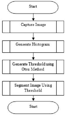
Fig.1.0. Typical sequence of steps in the image segmentation process using Otsu’s method.

• D.    Histograms for Content Based Image Retrieval

Various statistical analyses of histograms have also been used for other applications apart from contrast enhancement and image segmentation tasks For example Brunelli et al [20] used histograms analysis for image retrieval and Laaroussi et al [21] also used the concept of histogram in human tracking using colour-texture features and foreground-weighted histogram. Other efficient methods of classification of images and retrieval of images in a database using the images’ histogram have been proposed by [22-24]. Again, the histogram based methodology has been used in [25] for determination of the critical points condensation-evaporation systems.

• II.    Histogram Generation Process

The generation of the histogram typically takes two (2) steps and they are:

• 1.    The first step is to divide the range of values into a series of intervals (bin) of equal sizes. These intervals are consecutive, non-overlapping and adjacent.

• 2.    In the second step frequency of each bin is generated which is nothing but the number of values in each bin.

A grayscale image’s histogram generation process typically plots the frequency at which each gray-level occurs from 0 to 255. Histogram represents the frequency of occurrence of all gray-levels in the image, that means it tell us how the values of individual pixel in an image are distributed. The colour histogram generation approach uses a method relatively different from the grayscale even though values in all the three (3) channels such as what is found in the RGB (Red, Green, Blue) images are used as well. Figure 2.0 shows a grayscale image and its histogram.

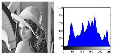
(a)                             (b)

Fig.2.0. (a) A grayscale image of Lena (b) Histogram of image (a)

The algorithm for the generation of histogram is illustrated below

Histogram

Let M be the number of Rows in the image

Let N be the number of Columns in the image

H(256) //A zero base index array

For x ^ 1 to M

For y ^ 1 to N

H(I(x,y)) ^ H(I(x,y)) + 1

End For

End For

//M holds the number of rows and N the number of columns in the image matrix.

• A.    Computational time complexity of histogram process

The time complexity of the histogram generation algorithm is proportional to the number of pixels to be processed. As the number of rows (M) in an image becomes approximately equal to that of the columns (N), M ≈ N, the computational time for constructing a histogram becomes O(N²) . The nature of the algorithm behaves so because all the pixels need to be traversed before the histogram can be constructed. The running time complexity for the algorithm therefore exhibits a quadratic time complexity with respect to the width of image. This makes the time expected to complete a task increases significantly as N increases. Fig 3.0 illustrates a graph depicting the quadratic nature of the running time of the algorithm as N increases.

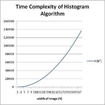
Fig.3.0. The quadratic running time complexity of histogram generation task.

In image processing and computer vision tasks where histograms are required, the total computational time to complete a task is greatly influenced by the sizes of the images. More time will be required to get the final task completed as the size of the image increases. If the time expected to complete the histogram generation is considerably reduced, then the overall computational time complexity taken by a lot of such algorithms can be reduced significantly and hence microcontrollers and low resourced computers can process images in real-time.

In order to reduce the computational time required to generate histogram, the total number of pixels needed to be accessed must be reduced. A way to do this is to select a subset of all the pixels that make up the image and use them to generate the histogram. The approximated histogram will be generated with limited number of pixels, but should have a close resemblance or be same as the actual one in terms of shape of the histograms or normalized histograms. This will make it possible for whatever statistical values that should have been generated on the actual histogram to be generated with the approximated histogram without any significant difference.

The neighbourhood concept which develops algorithms to take advantage of a pixel’s neighbourhood for estimating its value has been extensively used under the concept of local approximation. The local approximation technique has been explored in the design of image enhancement techniques such a filtering and image deblurring by using the idea of approximating a pixel’s value for better image. A typical filtering algorithm such as the median filtering and all the median based filtering algorithms [26-27] use the statistical median of a pixel’s neighbourhood to estimate or determine an ideal value for that particular pixel. This is done because the pixel value may be considered as a noise and these algorithms try to estimate what the actual value should be. These estimations of the pixels values are approximation of the original or actual image and the algorithms have generated images of acceptable quality.

• B.    Approximation of the histogram

One main aim for approximation of the histogram is to reduce the time expected to complete a task or process. For example, the sampling techniques used in statistical survey try to select a subset from a population and draw conclusions for the general population based on the results observed from the selected number. The need for reducing computational time for various image processing algorithms is necessary because it helps in making algorithms run in real time. Philips et al [28] used highly-accurate approximate histograms belonging to the equi-depth and compressed classes to avoid computing overheads when unnecessary. The method resulted in improving computational time expected to update records in a relational database significantly. Approximating a process as a way of satisfying time constraints that cannot be achieved through normal process was also discussed by [29-31], where approximate processes were adapted to solve problems in real-time. Segeev and Titova [32] described a fast method for computing Hu's image invariants. The invariants are found by approximation using generalized moments computed in a sliding window by a parallel recursive algorithm.

This paper proposes a new method that can be used to effectively generate an approximated histogram for most image processing and computer vision task that require histogram. The effectiveness of the method is based on reducing significantly the time expected for the generation of statistical values from a given image. The improved time complexity for the generation of these values, also significantly helps improve the time required by image processing and computer vision applications that depend on such values to get their task done successfully.

• III.    The Proposed Method for the Generation of Histogram

The method bases its assumption on the fact that given a pixel in an image, the pixel will have similar characteristics with its neighbours. This assumption makes it possible for a group of pixels to be represented by just one of the pixels. This assumption may not always be true especially at the instance where an image contains a lot of noise or edges or high texture, but generally true for a real world image.

The proposed algorithm uses a pixel to represent a group of pixels in an image and only the selected number of pixels is used to generate histogram for the image. Using a pixel in an image to represent w number of pixels will mean that an image of size M x N can be represented by (M.N)/w pixels. As w increases, the number of pixels that represents an image reduces and hence reduces the time expected to generate histogram for the image. A relatively high w may lead to lose of relevant information which may not give accurate results as expected. Also a small value for w may also result in computation time required to traverse the number of pixels selected equivalent to that of the actual histogram.

If we let Pt be a pixel that effectively represents w number of pixels, then Pt must have a value that can exhibit characteristic similar to all the members of the set it represents. Using a rectangular or square connected neighbourhood, we propose a kernel or window or subimage of size n x n in the given image as w .

Let w = n x n    for n = 3,5,7,9....N

The centre of the square window is selected as Pt because it is likely to exhibit characteristic that is common to all its neighbourhood values than any other pixel in the window. Fig 4.0 illustrates examples of various window sizes.

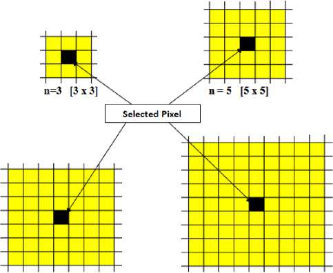
11=7 [7x7]                        n = 9 [9x9]

Fig.4.0. Illustration of various window sizes.

The entire window or kernel or sub-image will be represented by the central pixel. The efficacy of the output will generally depend on the nature of the values in a selected window and what the histogram will be used for. Most histograms generated by image processing tasks are further converted to Probability Density Function (PDF), Cumulative Density Function (CDF) or the histogram is normalized before they are used for other forms of statistical estimations. If the normalized histogram is required, then it is expected that the normalized histogram generated using the entire image will be equivalent to that of the approximated histogram.

The proposed histogram estimation algorithm

Function Histogram(Image Img)

//Img is a grayscale image with 256 levels (0 – 255)

//Img of Size M x N

// Let h be an array to store the approximated histogram. h(0:255) ^ 0 //Initialize all elements of Histogram with value zero.

// Let nh  be an array to store the normalized approximated histogram.

//Let the number of rows in a selected window be n . The size of the window will be n x n . w ^ n²

// In this example, n is set to 5, which means a pixel will be used to represent 25 pixels in the image n ^ 5

Start ^ (n+1)/2

For I <- Start To M Step n

For Start ^ Start To N Step n h(Img(I,J)) ^ h(Img(I,J)) +1

End For

End For

//Normalized Histogram (NH)

//Let Count be the total number of sub pixels that were used to represent the entire image

Count ^ round [(Mx N) / (n*n)]

For I = 0 To 255

nh(I) ^ h(I) / Count

End For

End Function

• IV.    Testing of Algorithm

The testing of the algorithm was done in two (2) main phases. The initial testing was done to evaluate the efficacy of the method by simply comparing the approximated histograms of images and their actual histograms. It was done by simply generating statistical values (Mean(µ), Variance, Standard Deviation, Maximum Value, Minimum Value, Median, Mode, and Entropy) using the approximated and the actual histograms and the percentage deviations of the approximated results from the actual results evaluated. Table 4.0 illustrates the average deviation results from several images that were used for the experiment. Again, the proposed method was analysed by using linear regression on the normalized histograms. The R-Squared values of the linear regression were computed using the two normalized histograms (actual and approximated histograms). The R-Squared value ranges between 0 and 1, and the higher the value, the better it is for one dataset to be used to predict the other. The final experiment in this phase tried to estimate the computation time of the proposed method and to establish that it can considerably reduce the time required to complete the histogram generation process. Two (2) methods were used for estimation of the time and they are the Big-O notation and CPU run time. The Big-O method estimates the time that an algorithm completes a task by counting the number of key operations. In this research, the number of iterations that is performed by the actual algorithm and the approximated algorithm is compared. The number of times the approximated runs faster than the actual is then recorded. The CPU’s run time estimation was done by subjecting both histograms generating methods to a particular system environment and the time taken to generate the actual and the approximated were recorded for comparison. A Processor with 1.6Hz (2 CPUs) and Memory of 4GB was used for this experiment. Due to the multitasking nature of computers today, the time at one point may be different when the same algorithm is run another time. As a result of this, algorithms were made to run 10,000 times on a particular image and the maximum, minimum, mean, and median times were registered.

The second phase of the testing of the proposed method substituted the actual histogram with the approximated method for the task of contrast enhancement and automatic threshold estimation. The Histogram Equalization (HE) for contrast enhancement and the Otsu’s automatic methods were specifically used for the experiments. The contrast enhancement technique was implemented using the actual histograms and the approximated histograms. The Peak Signal-to-Noise Ratio (PSNR) metric was then used to evaluate how close the two generated images were by comparing them to the original images used for the enhancement. This ratio is often used as a quality measurement between the original and a compressed image. The higher the value of PSNR, the better the quality of the compresed, or reconstructed image. The average percentage deviations of the approximated histogram’s PSNRs from the actual histogram’s PSNRs were computed to evaluate the efficacy of the proposed method. The formula for PSNR is as indicated by equations 3 and 4.

^ [ 1 1 ( m , n ) - 1 2 ( m , n ) ] 2

MSE = M , N ----------------- (3)

M * N

PSNR = 10log

( MSE J

The final set of experiments used the proposed histogram in place of the actual one for the Otsu’s automatic threshold estimation. If we assume that the capturing of image, generation of the histogram and the calculation of the automatic threshold takes time t 1 , t 2 and t 3 respectively, then the total time required for generating threshold value can be calculated by using equation 5.

Total time = t 1 + t 2 +t 3 (5)

It is important to reduce t2 considerably so that the total time expected to perform the estimation of threshold value will be reduced significantly. A window size of n = 7 is proposed for the estimation of the histogram and it is expected that the computational time complexity for the generation of the histogram will be O(MN/7.7) = O(MN/49). That is, the running time of the histogram generation component of the Otsu method will be 49 times faster than that of the classical histogram generation for a grayscale image. However, it must be stated that the histogram generation is just part of the sequence of tasks for estimation of the automatic threshold value.

The CPU time was used to evaluate the proposed computation time complexity. The Minkowski distance formula is used on the binarized images generated by the approximated and the actual thresholds. The percentage similarity as used by the distance formula is also indicated. Ten thousand (10,000) images were used for three (3) set of experiments. Image sizes of 128x85, 256x170, and 512x340 were used for the experiments. The Otsu automatic threshold generation methods that use 1D and 2D histograms were all used in this experiment.

• V.    Results and Discussions

• A.    Results of Statistical Values estimations

The following images in the Fig 5.0 were used for the statistical experiments and the results presented in Table 1.0.

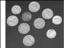
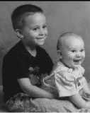
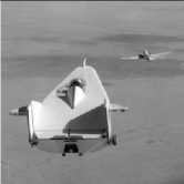
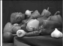
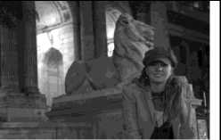
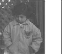
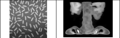
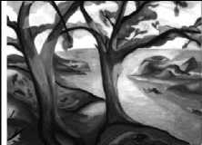
Fig.5.0. Sample images used for the initial experiments

Table 1.0.Average percentage deviations of various statistical values generated from the actual and approximated histograms.

	Approximated histogram using (n)
	3	7	11	15	19	21
Mean	0.09	0.41	0.55	1.06	1.44	1.47
Mode	0	0	0	0	0	0
Median	0	0	0	0	0	0
Max	0.36	0.49	0.93	1.31	3.02	5.13
Min	9.72	12.88	13.08	23.15	25.24	22.42
StDev	0.09	0.37	1.07	1.16	1.92	2.57
Variance	0.06	0.72	1.67	2.03	4	5.31

It was observed from Table 1.0 that the mean, mode, and median produced excellent results as n increases. This suggests that if these values are to be extracted from a histogram, it can efficiently be done even when a large value is selected for n. Standard deviation and Variance from the approximated method also produced very good result. The Max and Min though produced good results, their error margins increases with increasing n.

• B.    Linear Regression on Normalized Histograms

This test compared the normalized histograms using R-Squared test. Ten (10) different sizes of kernel or window were used for the experiment, and the normalized histogram for each instance of n was compared to the actual histogram. Plots of the actual and approximated histograms were generated for visual evaluate of the method. Continuous line in a plot represents the actual histogram, while the dotted ones represent the approximated histogram. Values of n=3, 5, 7, 9, 11, 13, 15, 17, 19, and 21 were used to generate ten (10) different approximated histogram. The cameraman image, as shown in fig 6.0, was used for this experiment. The result is shown in fig. 7.0

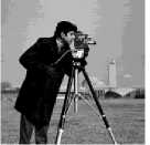
Fig.6.0. Cameraman 450 x 450

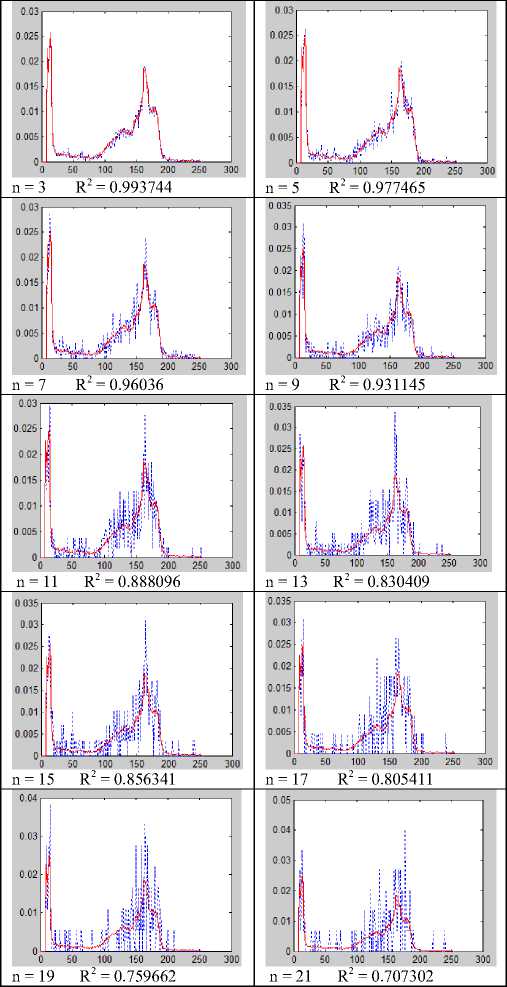
Fig.7.0. Plot of Actual Histogram and Approximated Histogram for various sizes of n

size was smaller than that of the pepper. Testpat1.png had the normalized approximated histogram having the same values as the actual histogram even when the selected kernel or window of 21 x 21 was used for a pixel. When such size of n is selected, it will theoretically make the algorithm run 441 times faster than the actual histogram generation method.

		R-Squared for window of size n
Image	Size	3	7	11	15	19	21
rice.png	256 x 256	0.99	0.953	0.89	0.808	0.721	0.721
pout.tif	240 x 291	0.998	0.984	0.963	0.915	0.889	0.872
coins.png	300 x 246	0.997	0.978	0.967	0.906	0.893	0.921
kids.tif	318 x 400	1	0.996	0.993	0.983	0.968	0.969
spine.tif	490 x 367	1	1	0.999	0.999	0.995	0.995
peppers.png	512 x 384	0.998	0.988	0.969	0.95	0.884	0.882
tape.png	512 x 384	0.998	0.99	0.973	0.957	0.93	0.923
testpat1.png	512 x 384	1	1	1	1	1	1
liftingbody.jpg	512 x 512	0.998	0.992	0.982	0.972	0.963	0.942
tree.tif	1400 x 1032	0.999	0.994	0.984	0.977	0.958	0.956
mandi.tif	3039 x 2014	1	0.999	0.999	0.997	0.995	0.995

• C.    Computational Time Complexities for various values of n

The Tables 3.0 and 4.0 illustrate various windows sizes and the estimated time expected to complete the generation of the histogram. The value indicates the speed of the proposed method as compared to that of the actual method for the generation of histogram. It was observed that the speed of the approximated method always outperformed that of the actual method’s time significantly.

n	3	5	7	9	11	13	15	17	19	21
Big-O	9	25	49	81	121	169	225	289	361	441

The proposed method was again applied on eleven (11) images of various sizes in the MatLab folder. Ten(10) n values were selected for each image and the normalized histogram of the selected pixels compared with the actual histogram. Table 2.0 illustrates the correlation values for the various window or kernel sizes selected for the approximation approach.

From the table 2.0 it was observed that when a window of 11 x 11 was selected for the approximated method, the method still exhibited a very good correlation with the actual histogram. It was observed generally that the nature of the pixel values distributions, size of the image and the window or kernel size influenced the outcome of the algorithm as illustrated in table 2.0. The Spine.tif with size 490 x 367 had the normalized approximated histogram much closer to the actual one even though its

Table 4.0. CPU Run Time Estimation

n	3	7	11	15	19	21
Minimum Speed	8.09	25.87	76.16	103.5	157.8	161.3
Median Speed	9.03	47.35	107.2	146.6	204.6	252.1
Mean Speed	8.98	45.58	105.7	156.2	219.5	281.4
Maximum Speed	9.68	53.05	119.3	209	308.9	393.3

• D.     Histogram Equalization (HE) for contrast

Enhancement

PSNR Differences in percentage from Table 5.0 are indication that histogram equalization for contrast enhancement can be effectively be done with high values of n. Figure 8.0 illustrates examples of results of histogram equalization for contrast enhancement for some selected images.

Table 5.0.Percentage deviations of using the approximated and actual histogram for contrast enhancement of images

	Approximated histogram using (n)
	3	7	11	15	19	21
PSNR Difference	0	0.03	0.06	0.11	0.13	0.17

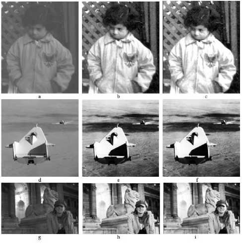
Fig.8.0. Sample images with contrast enhancement using Histogram Equalization (HE). (b) is the result of contrast enhancement using the actual histogram of image (a). Image (c) is the result of contrast enhancement using the approximated histogram with n = 11 of image (a). (e) is the result of contrast enhancement using the actual histogram of image (d). Image (f) is the result of contrast enhancement using the approximated histogram with n = 11 of image (d). (h) is the result of contrast enhancement using the actual histogram of image (g). Image (i) is the result of contrast enhancement using the approximated histogram with n = 11 of image (g).

• E.    Otsu Automatic Threshold Estimation using approximated histogram

The Actual and Approximated histograms of a given set of images were used for the Otsu automatic threshold generation. Table 6.0 illustrates the various average CPU times for generation of the threshold values.

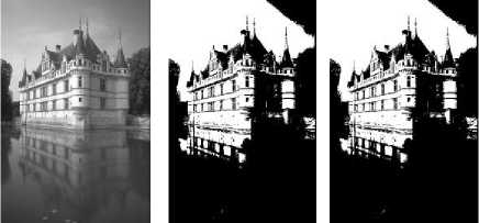
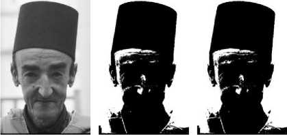
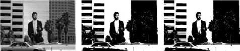
The results of the experiment indicated that the approximated can be effectively be used for automatic threshold estimation with an excellent results for n = 7. The approximated histogram made it possible for the overall time expected to generate an automatic threshold value using the Otsu 1D-histogram method to be completed 24 times faster than the actual histogram would have been used on an image of size 512 x 340.

A 256x256 2D-histogram of grayscale value and neighbourhood average grayscale value pair were generated using the classical method and the proposed partitioning method. Hundred (100) images from the Berkeley Segmentation Dataset and Benchmark images

Table 6.0. CPU running time of the estimation of Otsu automatic threshold (1D Histogram)

Images of 128x85 Images of size 256x170 Images of size 512x340 Actual Histogram Generation - Average Time in Seconds (A) 0.00260 0.01017 0.04412 Approximated Histogram Generation -Average Time in Seconds (B) 0.00007 0.00022 0.00092 Average Number of elements traversed -Actual Histogram (C) 11891 47567 190266 Average Number of Elements Traversed - Approximated Histogram (D) 242 969 3890 Average Time for 1D-Otsu Threshold Estimation Using Actual Histogram (E) 0.00092 0.00094 0.00103 Average Time for 1D-Otsu Threshold Estimation Using Approximated Histogram (F) 0.00085 0.00086 0.00095 Total Time for Estimating Threshold using the Actual Histogram (A+E) 0.00353 0.01110 0.04514 Total Time for Estimating Threshold using the Approximated Histogram (B+F) 0.00092 0.00108 0.00187 Average threshold value for Otsu using Actual Histogram 0.40157 0.39742 0.39750 Average threshold value for Otsu using Approximated Histogram 0.41040 0.39895 0.39611 Average PSNR 22.23751 25.26612 24.70694 Percentage similarity of segmented images using approximated and actual thresholds (Minkowski distance) 98.90669 99.80959 99.81807 Histogram Generation Speed of Approximated as compared to the Actual Method 38.82959 45.41497 47.92864 Threshold generation speed of Approximated method as compared to the actual method 3.83116 10.28708 24.19503 were used for this experiment. It was observed that the time expected to generate the 2D histogram using a partition of 7 x 7 sub-images resulted in average CPU running time of 47.5 times faster the traditional time required to generate a 2D-histogram. Again the overall time expected to generate the threshold value also reduced significantly to about 15 times faster than the original Otsu 2D-histgram method. When all the threshold values generated from the actual method and the approximated method were compared with the linear regression analyses, the R-Squared was 0.995911. The values indicated that the proposed method was excellent in generating threshold values and also performing at an excellent speed. Fig 9.0 illustrates some sample images and their binary images after both histograms were applied for segmentation.

a               b                c

d               e              f

g                  h                   i

Fig.9.0. Sample images and results after the application of the automatic threshold method. The b, e and h used the actual histograms for threshold generation and c, f and i used the approximated histograms.

• VI.    Conclusion

The paper proposes a new method for faster generation of image’s histogram. The need for fast histogram generation is as a result of the fact that a lot of image preprocessing tasks require this in order to get their tasks done. The paper proposes that, the central pixels of a kernel be used to represent the whole kernel. Logically what this means is that an image is partitioned into several sub-images and each sub image is represented using just a pixel. This approach reduces the number of pixels to be traversed during the histogram generation, hence, the computational time complexity of generating histogram. The experimental results show that for n=3,5,7,9, and 11 the computation time expected to generate histogram or normalized histogram can be reduced considerably and also produce excellent results for extracting common statistical values from the histogram. Contrast enhancement using histogram equalization (HE) and Otsu 1D and 2D automatic threshold estimation time for completion can be extremely improved with this method with equivalent results. If an ideal n is selected for a window (n x n) then the algorithm will be n2 time faster than the traditional method of generating the histogram which makes it good for real-time application.

• VII.    Future Work

The results of the experiments indicated that the proposed algorithm’s outcome does not solely depend on the size of the image, but also the nature of the distribution of pixel’s values in an image. Future work will consider various image categories such as road traffic conditions, settlements, banking scenes, etc in order to determine which size of window will be ideal for various scenarios for the purposes of real-time implementation. This will enable developers to set n based on the kind of scene that they wish to apply the proposed method. Again the experiments in this research focused on only grayscale images and therefore future work will consider the colour histograms and the use of the approximated method for other image processing algorithms or models that will require a histogram.