Feature Based Audio Steganalysis (FAS)

Steganography is the art and science of hiding information by embedding messages with in other seemingly harmless messages. Steganography means “covered writing” in Greek. As the goal of steganography is to hide the presence of a message and to create a covert channel, it can be seen as the complement of cryptography, whose goal is to hide the content of a message. To achieve secure and undetectable communication, stego-objects, documents containing a secret message, should be indistinguishable from cover-objects, documents not containing any secret message. In this respect, steganalysis is the science of detecting hidden information. The main objective of steganalysis is to break steganography and the detection of stego carrier is the goal of steganalysis. Steganalysis itself can be implemented in either a passive warden or active warden style. The passive warden simply examines the message and tries to determine if it potentially contains hidden information or not. An active warden can alter messages deliberately, even though there may not be any trace of hidden information, in order to foil any secret communication. Almost all digital file formats can be used for steganography, but the image and audio files are more suitable because of their high degree of redundancy [1, 2]. Fig. 1 below shows the different categories of file formats that can be used for steganography techniques.

Figure 1: Types of Steganography

Among them image steganography is the most popular of the lot. In this method the secret message is embedded into an image as noise to it, which is nearly impossible to differentiate by human eyes [3, 4, 5]. In video steganography, same method may be used to embed a message [6, 7, 8]. Audio steganography embeds the message into a cover audio file as noise at a frequency out of human hearing range [9]. One major category, perhaps the most difficult kind of steganography is text steganography or linguistic steganography [1, 10]. The text steganography is a method of using written natural language to conceal a secret message as defined by Chapman et al. [11].

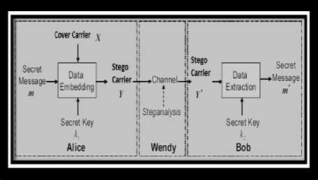
Figure 2: Generic Steganography and Steganalysis

In this article , a novel feature based audio steganalyser has been proposed which takes several audio quality measures namely statistical moments, invariant moments, entropy, signal-to-noise ratio (SNR) and Czenakowski distance as features for the design of steganalyser. Audio quality metric will act as a functional unit that converts its input signal into a measure that supposedly is sensitive to the presence of a steganographic message embedding. This steganalyzer searches for the measures that reflect the quality of distorted or degraded audio signal vis-à-vis its original in an accurate, consistent and monotonic way. Such a measure, in the context of steganalysis, should respond to the presence of hidden message with minimum error, should work for a various embedding methods, and its reaction should be proportional to the length of the hidden message.

This paper has been organized as following sections: Section II describes some review works of audio steganography. Section III reviews the previous work on audio steganalysis. Section IV describes the various methods for audio feature selection. Experimental Results of the method has been discussed in Section V and Section VI draws the conclusion.

• II.    Review of related works on audio STEGANOGRAPHY

This section presents some existing techniques of audio data hiding namely Least Significant Bit Encoding, Phase Coding Echo Hiding and Spread Spectrum techniques. There are two main areas of modification in an audio for data embedding. First, the storage environment, or digital representation of the signal that will be used, and second the transmission pathway the signal might travel [4, 11].

• A.    Least Significant Bit Encoding

The simple way of embedding the information in a digital audio file is done through Least significant bit (LSB) coding. By substituting the least significant bit of each sampling point with a binary message bit, LSB coding allows a data to be encoded and produces the stego audio. In LSB coding, the ideal data transmission rate is 1 kbps per 1 kHz. The main disadvantage of LSB coding is its low embedding capacity. In some cases an attempt has been made to overcome this situation by replacing the two least significant bits of a sample with two message bits. This increases the data embedding capacity but also increases the amount of resulting noise in the audio file as well. A novel method of LSB coding which increases the limit up to four bits is proposed by Nedeljko Cvejic et al. [13, 14]. To extract secret message from an LSB encoded audio, the receiver needs access to the sequence of sample indices used during the embedding process. Normally, the length of the secret message to be embedded is smaller than the total number of samples done. There is other two disadvantages also associated LSB coding. The first one is that human ear is very sensitive and can often detect the presence of single bit of noise into an audio file. Second disadvantage however, is that LSB coding is not very robust. Embedded information will be lost through a little modification of the stego audio.

• B.    Phase Coding

Phase coding [8, 14] overcomes the disadvantages of noise induction method of audio steganography. Phase coding designed based on the fact that the phase components of sound are not as perceptible to the human ear as noise is. This method encodes the message bits as phase shifts in the phase spectrum of a digital signal, achieving an inaudible encoding in terms of signal-to-noise ratio. In figure 3 below original and encoded signal through phase coding method has been presented.

Original

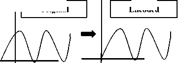
Encoded

Figure 3: The original signal and encoded signal of phase coding technique .

Phase coding principles are summarized as under:

• •    The original audio signal is broken up into smaller segments whose lengths equal the size of the message to be embedded.

• •    Discrete Fourier Transform (DFT) is applied to each segment to create a matrix of the phases and Fourier transform magnitudes.

• •    Phase differences between adjacent segments are calculated next.

• •    Phase shifts between consecutive segments are easily detected. In other words, the absolute phases of the segments can be changed but the relative phase differences between adjacent segments must be preserved.

Thus the secret message is only inserted in the phase vector of the first signal segment as follows:

phasenew =

— if message bit is 0

Я

— — if message bit is 1

• •    A new phase matrix is created using the new phase of the first segment and the original phase differences.

• •    Using the new phase matrix and original magnitude matrix, the audio signal is reconstructed by applying the inverse DFT and by concatenating the audio segments.

To extract the secret message from the audio file, the receiver needs to know the segment length. The receiver can extract the secret message through different reverse process.

The disadvantage associated with phase coding is that it has a low data embedding rate due to the fact that the secret message is encoded in the first signal segment only. This situation can be overcome by increasing the length of the signals segment which in turn increases the change in the phase relations between each frequency component of the segment more drastically, making the encoding easier to detect.

• C.    Echo Hiding

In echo hiding [14, 15, 16] method information is embedded into an audio file by inducing an echo into the discrete signal. Like the spread spectrum method, Echo Hiding method also has the advantage of having high embedding capacity with superior robustness compared to the noise inducing methods. If only one echo was produced from the original signal, only one bit of information could be encoded. Therefore, the original signal is broken down into blocks before the encoding process begins. Once the encoding process is completed, the blocks are concatenated back together to form the final signal. To extract the secret message from the final stego audio signal, the receiver must be able to break up the signal into the same block sequence used during the encoding process. Then the autocorrelation function of the signal's cepstrum which is the Forward Fourier Transform of the signal's frequency spectrum can be used to decode the message because it reveals a spike at each echo time offset, allowing the message to be reconstructed.

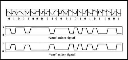
Figure 4: Echo Hiding Methodology

• D.    Spread Spectrum

Spread Spectrum (SS) [14] methodology attempts to spread the secret information across the audio signal's frequency spectrum as much as possible. This is equivalent to a system using the LSB coding method which randomly spreads the message bits over the entire audio file. The difference is that unlike LSB coding, the SS method spreads the secret message over the audio file's frequency spectrum, using a code which is independent of the actual signal. As a result, the final signal occupies a more bandwidth than actual requirement for embedding. Two versions of SS can be used for audio steganography one is the direct sequence where the secret message is spread out by a constant called the chip rate and then modulated with a pseudo random signal where as in the second method frequencyhopping SS, the audio file's frequency then interleaved with the cover-signal spectrum is altered so that it hops rapidly between frequencies. The Spread Spectrum method has a more embedding capacity compared to LSB coding and phase coding techniques with maintaining a high level of robustness. However, the SS method shares a disadvantage common with LSB and parity coding that it can introduce noise into the audio file at the time of embedding.

• III.    Review of related works on audio STEGANALYSIS

Audio steganalysis is very difficult due to the existence of advanced audio steganography schemes and the very nature of audio signals to be high-capacity data streams necessitates the need for scientifically challenging statistical analysis [29].

• A.    Phase and Echo Steganalysis

Zeng et. al [17] proposed steganalysis algorithms to detect phase coding steganography based on the analysis of phase discontinuities and to detect echo steganography based on the statistical moments of peak frequency [18]. The phase steganalysis algorithm explores the fact that phase coding corrupts the extrinsic continuities of unwrapped phase in each audio segment, causing changes in the phase difference [19]. A statistical analysis of the phase difference in each audio segment can be used to monitor the change and train the classifiers to differentiate an embedded audio signal from a clean audio signal.

• B.    Universal Steganalysis based on Recorded Speech

Johnson et. al [20] proposed a generic universal steganalysis algorithm that bases it study on the statistical regularities of recorded speech. Their statistical model decomposes an audio signal (i.e., recorded speech) using basis functions localized in both time and frequency domains in the form of Short Time Fourier Transform (STFT). The spectrograms collected from this decomposition are analyzed using non-linear support vector machines to differentiate between cover and stego audio signals. This approach is likely to work only for high-bit rate audio steganography and will not be effective for detecting low bit-rate embeddings.

• C.    Use of Statistical Distance Measures for Audio Steganalysis

H. Ozer et. al [21] calculated the distribution of various statistical distance measures on cover audio signals and stego audio signals vis-a-vis their versions without noise and observed them to be statistically different. The authors employed audio quality metrics to capture the anomalies in the signal introduced by the embedded data. They designed an audio steganalyzer that relied on the choice of audio quality measures, which were tested depending on their perceptual or non-perceptual nature. The selection of the proper features and quality measures was conducted using the (i) ANOVA test [22] to determine whether there are any statistically significant differences between available conditions and the (ii) SFS (Sequential Floating Search) algorithm that considers the inter-correlation between the test features in ensemble [23]. Subsequently, two classifiers, one based on linear regression and another based on support vector machines were used and also simultaneously evaluated for their capability to detect stego messages embedded in the audio signals.

• D.    Audio Steganalysis based on Hausdorff Distance (HSDMHD)

The audio steganalysis algorithm proposed by Liu et. al [24] uses the Hausdorff distance measure [25] to measure the distortion between a cover audio signal and a stego audio signal. The algorithm takes as input a potentially stego audio signal x and its de-noised version x as an estimate of the cover signal. Both x and x are then subjected to appropriate segmentation and wavelet decomposition to generate wavelet coefficients [26] at different levels of resolution. The Hausdorff distance values between the wavelet coefficients of the audio signals and their de-noised versions are measured. The statistical moments of the Hausdorff distance measures are used to train a classifier on the difference between cover audio signals and stego audio signals with different content loadings.

• E.    Audio Steganalysis for High Complexity Audio Signals

  More recently, Liu et. al [28] propose the use of stream data mining for steganalysis of audio signals of high complexity. Their approach extracts the second order derivative based Markov transition probabilities and high frequency spectrum statistics as the features of the audio streams. The variations in the second order derivative based features are explored to distinguish between the cover and stego audio signals. This approach also uses the Mel-frequency cepstral coefficients [29], widely used in speech recognition, for audio steganalysis. Recently two new methods of audio steganalysis of spread spectrum information hiding have been proposed in [3132].

• IV.    Audio feature selection

In this section several audio quality measures in terms of statistical and invariant moments up to 7 ^th order and entropy, signal-to-noise ratio (SNR) and Czenakowski distance has been investigated for the purpose of audio steganalysis. Various moments and other features of the audio signals are sensitive to the presence of a steganographic message embedding. Moments based features have been extracted for steganalytic measure in such a way that reflect the quality of distorted or degraded audio signal vis-à-vis its original in an accurate, consistent and monotonic way. Such a measure, in the context of steganalysis, should respond to the presence of hidden message with minimum error, should work for a large variety of embedding methods, and its reaction should be proportional to the embedding strength.

• A.    Moments based Audio feature

To construct the features of both cover and stego or suspicious audios moments [30] of the audio series has been computed. In mathematics, a moment is, loosely speaking, a quantitative measure of the shape of a set of points. The "second moment", for example, is widely used and measures the "width" (in a particular sense) of a set of points in one dimension or in higher dimensions measures the shape of a cloud of points as it could be fit by an ellipsoid. Other moments describe other aspects of a distribution such as how the distribution is skewed from its mean, or peaked. There are two ways of viewing moments [30], one based on statistics and one based on arbitrary functions such as f(x) or f(x, y). As a result moments can be defined in more than one way.

Moments are the statistical expectation of certain power functions of a random variable. The most common moment is the mean which is just the expected value of a random variable as given in 1.

µ = E[ X ] =^∞ ∫ x f ( x ) dx

-∞ (1)

where f ( x ) is the probability density function of continuous random variable X . More generally, moments of order p = 0, 1, 2, … can be calculated as m p = E [ X^p ].These are sometimes referred to as the raw moments. There are other kinds of moments that are often useful.

One of these is the central moments µ p = E [( X – µ ) ^p ].The best known central moment is the second, which is known as the variance given in 2.

σ2 = (x-µ)2 f (x)dx = m -µ2

Two less common statistical measures, skewness and kurtosis, are based on the third and fourth central moments. The use of expectation assumes that the pdf is known. Moments are easily extended to two or more dimensions as shown in 3.

mpq=E[XpYq]=∫∫xpyq f(x,y)dxdy

Here f ( x , y ) is the joint pdf.

However, moments are easy to estimate from a set of measurements, x i . The p -th moment is estimated as given in 4 and 5.

1N m= pN ∑i=1

(Often 1/ N is left out of the definition) and the p -th central moment is estimated as

µ p = ¹ ∑ ( x i - x ) ^p

N i(5)

X is the average of the measurements, which is the usual estimate of the mean. The second central moment gives the variance of a set of data s2 = µ2.For multidimensional distributions, the first and second order moments give estimates of the mean vector and covariance matrix. The order of moments in two dimensions is given by p+q, so for moments above 0, there is more than one of a given order. For example, m20, m11, and m02 are the three moments of order 2.

This view is not based on probability and expected values, but most of the same ideas still hold. For any arbitrary function f ( x ), one may compute moments using the equation 6 or for a 2-D function using 7.

да

mp = J xp f (x) dx

-да

mpq = JJ xp yq f(x, У)dx dy

Notice now that to find the mean value of f ( x ), one must use m 1 / m 0 , since f ( x ) is not normalized to area 1 like the pdf. Likewise, for higher order moments it is common to normalize these moments by dividing by m 0 (or m 00 ). This allows one to compute moments which depend only on the shape and not the magnitude of f ( x ). The result of normalizing moments gives measures which contain information about the shape or distribution (not probability dist.) of f ( x ).

For digitized data (including images) we must replace the integral with a summation over the domain covered by the data. The 2-D approximation is written in 8.

MN

mpq =EZ f(x, j xp yqq i=1 j=1

MN

= ££ f (i, j) iT

‘ = 1 j = 1                                                       (8)

If f ( x , y ) is a binary image function of an object, the area is m 00 , the x and y centroids are ^x = m io / ^m oo and y = ^m oi / m oo .

In many applications such as shape recognition, it is useful to generate shape features which are independent of parameters which cannot be controlled in an image. Such features are called invariant features. There are several types of invariance. For example, if an object may occur in an arbitrary location in an image, then one needs the moments to be invariant to location. For binary connected components, this can be achieved simply by using the central moments, ^ pq . If an object is not at a fixed distance from a fixed focal length camera, then the sizes of objects will not be fixed. In this case size invariance is needed. This can be achieved by normalizing the moments as given in 9.

u

П pq =    , where Y = ? P + q) +1.

^{U o0}                                           (9)

The third common type of invariance is rotation invariance. This is not always needed, for example if objects always have a known direction as in recognizing machine printed text in a document. The direction can be established by locating lines of text.

M.K. Hu derived a transformation of the normalized central moments to make the resulting moments rotation invariant as given in 10.

p + q = 2

Ф\ = to + %2

Фг = (№ - W + 4^n p+q = 3

Ф1 = (to - 3j/i2)² + (№ - ^to)¹

Фа = (to +1/12)² + (to + Ч21)²

Ф5 = (чзо - 3?ji2)(to + rj_l2)[(to + to)² - 3(;j2i + r/03)²]

+ (to - ЗЦ21Х403 + S2i)[(to + ^2i)~ - 3(i;i2 + to)1]

Фб = (to - toJK'/so + to)² - (^21 + to)²]

+4ijn(to + t/i2)(to + I)2i)

Ф1 = (3i)2i - toll'Jw + 'Ji2)[(43u + to)² - 3(i?2i + to)²] + (1)30 - 31Jl2)(l)2l + to)l(to + 1)21 )² - 3( 1)31) + 1)12)*]

• B.    Entropy based audio features

  In information theory, Entropy is a measure of the uncertainty associated with a random variable. In this context, the term usually refers to the Shannon Entropy, which quantifies the expected value of the information contained in a message, usually in units such as bits. In this context, a 'message' means a specific realization of the random variable. Equivalently, the Shannon Entropy is a measure of the average information content one is missing when one does not know the value of the random variable. The concept was introduced by Claude E. Shannon [33] in his 1948 paper "A Mathematical Theory of Communication”.

Named after Boltzmann's H-theorem, Shannon denoted the entropy H of discrete random variable X with possible values { x 1 , ... , x n } as,

нт=E(/(x)>

Here E is the expected value, and I is the information content of X . I ( X ) itself a random variable. If p denotes the probability mass function of X then the entropy can explicitly be written as

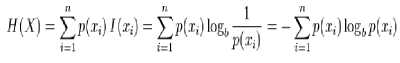
where b is the base of the logarithm used. Common values of b are 2, Euler's number e, and 10, and the unit of entropy is bit for b = 2, nat for b = e, and dit (or digit) for b = 10.

• C.    Signal to Noise ratio (SNR)

Signal-to-noise ratio or SNR [41] is a measure used in science and engineering that compares the level of a desired signal to the level of background noise. It is defined as the ratio of signal power to the noise power. A ratio higher than 1:1 indicates more signal than noise. Although SNR is mainly quoted for electrical signals but it can also be applied to any other form of the signal. The signal-to-noise ratio, the bandwidth, and the channel capacity of a communication channel are based on the Shannon–Hartley theorem.  Signal-to-noise ratio is defined as the power ratio between a signal (meaningful information) and the background noise (unwanted signal):

SNR=(P signal /P noise )

If the signal and the noise are measured across the same impedance, then the SNR is the square of the amplitude ratio:

SNR=(P signal /P noise )=(A signal /A noise )

i = 1

where x(i) is the original audio signal, y(i) is the distorted audio signal

• D.    Czenakowski Distance(CZD)

CZD (Czenakowski Distance) as PSNR is a per-pixel quality metric (it estimates the quality by measuring differences between pixels). Described in literature as being “useful for comparing vectors with strictly nonnegative elements” it measures the similarity among different samples. This different approach has a better correlation with subjective quality assessment than PSNR. This is a correlation-based metric [34, 41], which compares directly the time domain sample vectors

1 у f i - ²*min( x ( i ), У ( i )) ) N £<       x ( i ) + У ( i )    J

• V.    Design of audio steganalyser

The Steganalysis technique proposed here to test the presence of the hidden message is the combination of statistical moments and invariant moments based analysis along with several other audio features on the cover data and stego data series for the estimation of the presence of the secret message as well as the predictive size of the hidden message. Steganalysis approach has been designed here based on the above mentioned fact considering cover audio data as the independent data series and stego audio data as the dependent series data. From the experimental results it can be shown that with the introduction of secret message/increasing length of the secret message moments parameters also changes. This is the basis of proposed steganalyzer that aims to classify audio signal as original and suspicious. In order to classify the signals as “cover” or “stego” based on the selected audio quality features, authors tested and compared three types of classifiers, namely, k- nearest neighbor classifier, support vector machines and back propagation neural network classifier.

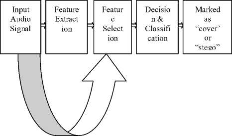
Figure 5: Block Diagram of the proposed steganalysis system

• a)    Support Vector Machine Classifier

In machine learning, support vector machines ( SVMs , also support vector networks ) are supervised learning models with associated learning algorithms that analyze data and recognize patterns, used for classification and regression analysis. The basic SVM takes a set of input data and predicts, for each given input, which of two possible classes forms the input, making it a non-probabilistic binary linear classifier. Given a set of training examples, each marked as belonging to one of two categories, an SVM training algorithm builds a model that assigns new examples into one category or the other. An SVM model is a representation of the examples as points in space, mapped so that the examples of the separate categories are divided by a clear gap that is as wide as possible. New examples are then mapped into that same space and predicted to belong to a category based on which side of the gap they fall on. In addition to performing linear classification, SVMs can efficiently perform non-linear classification using what is called the kernel trick, implicitly mapping their inputs into highdimensional feature spaces.

The support vector method works on principle of multidimensional function optimization [40], which tries to minimize the experiential risk i.e. the training set error. For the training feature data ( f_t , g_t ) , i = 1,.., N , g i G [-1,1], the feature vector F lies on a hyperplane given by the equation W T F + b = 0 , where w is the normal to the hyperplane.

The set of vectors will be optimally separated if they are separated without error and the distance between the closest vectors to the hyperplane is maximal.

A separating hyperplane in canonical form, for the i ^th feature vector and label, must satisfy the following criteria:

g_z .[( wF> b ] > 1, г = 1,2,.... N               (17)

The distance d(w, b; F) of a feature vector F from the hyperplane (w, b) given by,

IwT F + bl d (w, b; F) =                                   (18)

w

The optimal hyperplane can be achieved by maximizing this margin.

• b)    K Nearest Neighbor (KNN) Classifier

In pattern recognition,    the k-nearest    neighbor algorithm (kNN) is a method for classifying objects based on closest training examples in the feature space. K-NN is a type of instance-based learning, or lazy learning where the function is only approximated locally and all computation is deferred until classification. The k-nearest neighbor algorithm is amongst the simplest of all machine learning algorithms: an object is classified by a majority vote of its neighbors, with the object being assigned to the class most common amongst its k nearest neighbors (k is a positive integer, typically small). If k = 1, then the object is simply assigned to the class of its nearest neighbor. The same method can be used for regression, by simply assigning the property value for the object to be the average of the values of its k nearest neighbors. It can be useful to weight the contributions of the neighbors, so that the nearer neighbors contribute more to the average than the more distant ones. (A common weighting scheme is to give each neighbor a weight of 1/d, where d is the distance to the neighbor. This scheme is a generalization of linear interpolation.).The neighbors are taken from a set of objects for which the correct classification (or, in the case of regression, the value of the property) is known. This can be thought of as the training set for the algorithm, though no explicit training step is required. The k-nearest neighbor algorithm is sensitive to the local structure of the data. Nearest neighbor rules in effect compute the decision boundary in an implicit manner. It is also possible to compute the decision boundary itself explicitly, and to do so in an efficient manner so that the computational complexity is a function of the boundary complexity.

• c)    Back Propagation Feed Forward Neural Network Classifier

Any successful pattern classification methodology [38] depends heavily on the particular choice of the features used by that classifier .The Back-Propagation is the best known and widely used learning algorithm in training multilayer feed forward neural networks. The feed forward neural net refer to the network consisting of a set of sensory units (source nodes) that constitute the input layer, one or more hidden layers of computation nodes, and an output layer of computation nodes .The input signal propagates through the network in a forward direction, from left to right and on a layer-by-layer basis. Back propagation is a multi-layer feed forward, supervised learning network based on gradient descent learning rule. This BPN provides a computationally efficient method for changing the weights in feed forward network, with differentiable activation function units, to learn a training set of input-output data. Being a gradient descent method it minimizes the total squared error of the output computed by the net. The aim is to train the network to achieve a balance between the ability to respond correctly to the input patterns that are used for training and the ability to provide good response to the input that are similar. A typical back propagation network of input layer, one hidden layer and output layer is shown in figure 6.

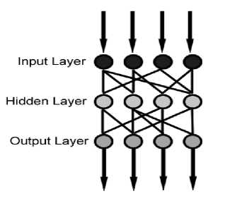
Figure 6: Feed Forward BPN

The proposed neural network based classifier is a two-layer feed-forward network, with sigmoid hidden and output neurons can classify vectors arbitrarily well, given enough neurons in its hidden layer. The network will be trained with scaled conjugate gradient back propagation.

• d)    Proposed Algorithm for Classification:

• •    Input: 30 Audio signals for training and 20 audio signals for testing

• •    Select the audio signals and extract various

features

• •    Embed secret  message based on five

steganography tools ( S–Tools, Our Secret, Steganography V 1.1, Silent Eye, Xiao Steganography)

• •    Repeat step 2 for stego audios also.

• •    Store the results

• •    Create a sample data set based on the results.

• •    Create training data set for identifying

cover/stego (cover=1, stego=0)

• •    Create training data set for identifying type of audio signal (out of 10 different types of audio signals)

• •    Test for classification and group them.

• •    Evaluate the performance of classifier based on ROC and Confusion Matrix

VI. Experimental results

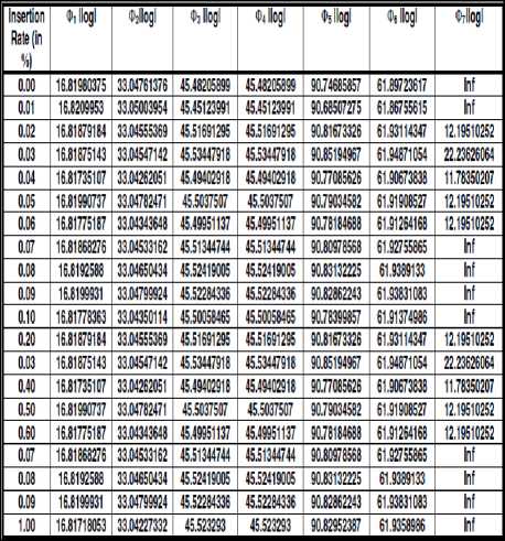
The steganalyzer has been designed based on a training set and using various audio steganographic tools. The steganographic tools used here Our Secret [44], S-Tools [42]., Steganography V 1.1, Silent Eye [45] and Xiao Steganography [43] .In the experiments 30 audio signals were used for training and 20 audio signals for testing. After embedding secret message into the cover audio with the various embedding rate rates of 0.01%,0.02% ,….,0.1% with 1% in increments and from 10% to 100% with 10% increments at various Stego audios has been created. Several audio quality measure parameters namely statistical moments, invariant moments, entropy, signal-to-noise ratio (SNR) and Czenakowski distance are used as features of these Stego audio signals. From table 1 and table 2 it can be seen that with the introduction of small message all the statistical moments’ value and invariant moments values changes. Table 3 shows the changes of different audio features at different embedding rate.

Insertion Rate H	UOIIogl	Ulllogl	U2llogl	UOIIogl	Ullogl	№llogl	lilfllogl	M7llogl
0.00	0.00000000	Ini	5.01434726	10.76686508	6.7920018!	18.05804036	7.58961747	9.55279478
0.01	0.00000000	lol	5.01436606	Ш.П155900	6.79327040	18.05066205	7.59052845	9.94602030
0.02	0.00000000	lol	5.01436713	10.77566326	6.79321801	10.05140694	7.5904ЛВ8	9.94628761
0.03	0.00000000	Ini	5.01436179	10.78205865	6.79310330	10.05455681	7.59021636	9.94863093
0.04	0.00000000	Ini	5.01437881	10.70545013	6.79300634	10.05560905	7.59020823	9.9489964
0.05	0.00000000	Ini	5.01435116	10.78576513	6.7929362!	10.05783700	7.58973018	9.95271517
0.06	0.00000000	Ini	5.01431625	10.78437928	S.7928!126	10.05762141	7.51970062	9.95270223
0.0?	0.00000000	Ini	5.01435375	10.78262711	6.79309417	10.05471134	7.59022919	9.94869163
0.00	0.00000000	Ini	5.01429762	10.78072779	6.79296125	10.05383546	7.5 9006319	9.94794204
0.09	0.00000000	Ini	5.01403524	10.77930259	6.79307585	10.05428190	7.59023374	9.94655996
0.10	0.00000000	Ini	5.01434330	'0 77903637	6.79311535	10.05393180	7.59026419	9.94835686
0.20	0.00000000	Ini	5.01430666	10.Л689911	6.79299598	10.05318137	7.59010105	9.94772815
0.03	0.00000000	Ini	5.01431966	10.78323382	6.79307192	10.05464313	7.59023999	9.94866184
0.40	0.00000000	Ini	5.01434505	10.76533458	6.79298501	10.05155689	7.51985122	9.95341726
0.50	0.00000000	Ini	5.01435076	10.76218531	6.79310704	10.05502114	7.59025561	9.94882058
0.60	0.00000000	Ini	5.01436439	10.79064476	6.79296899	10.05 963130	7.58982116	9.95376981
0.0?	0.00000000	Ini	5.01433211	10.78078636	6.79306011	10.05450815	7.59021489	9.94861504
0.06	0.00000000	Ini	5.01433795	10.79074527	6.79290477	10.05968878	7.51976742	9.95387044
0.09	0.00000000	Ini	5.01438906	10.76964552	6.79302935	10.05906084	7.51987617	9.95359105
1.00	0.00000000	Ini	5.01433926	10.79685680	6.79299135	10.06095969	7.58985409	9.95438418

Insertion Rate (in %)	Entropy	SNR	CZD
0.00	2.45516738	Inf	0
0.01	2.4557034	45.18973489	-0.013884068
0.02	2.45598777	45.33964251	-0.013406686
0.03	2.45575943	45.05233678	-0.014323239
0.04	2.45590419	45.17425201	-0.013934345
0.05	2.45603423	45.16653122	-0.013956717
0.06	2.45601392	44.91915257	-0.014788348
0.07	2.45611587	44.90460333	-0.014829142
0.08	2.45627255	44.89734694	-0.014853572
0.09	2.45594886	44.9778419	-0.014581887
0.10	2.45587288	44.97046222	-0.01460053
0.20	2.4561197	44.52248335	-0.016196642
0.30	2.4563804	44.56257236	-0.016060568
0.40	2.45609567	44.74769827	-0.015376221
0.50	2.45611056	44.64387791	-0.015756433
0.60	2.45607595	44.68510871	-0.01559517
0.70	2.45629909	44.65072259	-0.015725766
0.80	2.4560906	44.35931823	-0.016817145
0.90	2.45652286	44.42385054	-0.01658062
1.00	2.45623676	44.45647988	-0.016446308

In order to calculate the performance of three classifiers at different embedding rate and to show the relationship between the false-positive rate and the detection rate, authors have also calculated the receiver operating characteristics (ROC) curves of steganographic data embedding for the five different embedding methods. The ROC curves are calculated for the classifiers by first designing a classifier and then testing the data unseen to the classifier against the trained classifier. The testing results also consists of true positive (TP), true negative (TN), false positive (FP), and false negative (FN). The testing accuracy is calculated by (TP+TN) /

(TP+TN+FP+FN).Figure 7 – 12 shows the ROC analysis at different embedding rate for S Tools. Performance comparison of different classifier at various embedding rate has been shown in table 4. A comparative study amongst various existing audio steganalysis method with feature based steganalysis method has been shown in table 5.

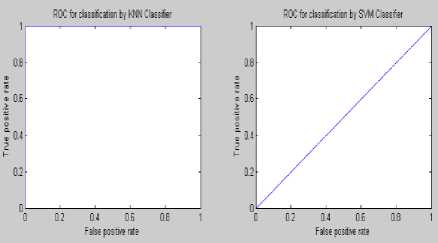
Figure7: ROC curve of steganalysis of S Tools at embedding rate 0.01%

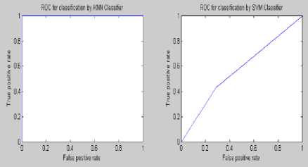
Figure 8: ROC curve of steganalysis of S Tools at embedding rate 0.02%

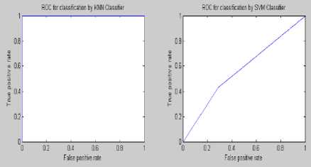
Figure 9: ROC curve of steganalysis of S Tools at embedding rate 0.03%

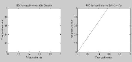
Figure 10: ROC curve of steganalysis of S Tools at embedding rate 0.04%

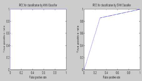
Figure 11: ROC curve of steganalysis of S Tools at embedding rate 0.05%

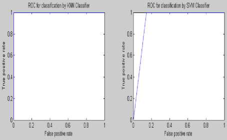
Figure 12: ROC curve of steganalysis of S Tools at embedding rate 0.1%

Table 4: Performance Analysis of different Classifier at various embedding rate

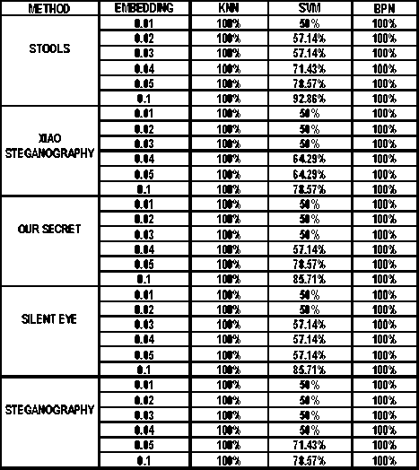
Table 5: Comparison among various audio steganalyser

Method

Audio steganalysis based on "negative resonance phenomenon|35

A Novel Audio Steganalysi s based on Higher-Order

Statistics of a Distortion

Measure with

Hausdorff Dlstance|36

Audio Steganalysis with Content-Independent Distortion Measures[37|

Qingzhong

Lluetal|38]

Feature based SteganalysisiFASi

No of Audio Stcganogr phy tools for Testing

No of classifier used for training and testing

Minimum embedding detection

ROC analysis incorporat ed

Aurracy Rate (In %)

Three tools used

Hlde4PGP,

Stegowav, STools

One (SVM Classifier)

60%

No

96.8% (Hlde4PGP), 98.6% (Stegowav).

85.6% (STook)

Steghide

One I SVM Classifier)

10%

Yes

80% (at emb rate 30%)

85% (at emb rate 50%)

90% (at emb rate 100%)

One (Linear reRression i

10%

Yes

Stefanos

Hide

4PG

STEGHI DE

Three tools .Hided PGP.l mlsible Secret,STools

Five tools used STOOLS, XIAO STEGANOGRAPH Y, OUR SECRET, SILENT EYE, STEGANOGRAPH

SVM

10%

Yes

Three (KNN,SVM,BPN)

1%

Yes

More

60% at 10%

80% al 50%

at

10% икс.

at

60% at 10% emb than 90% at 50% emb rate.

100% at 100% emb rate.

99.1% (Hlde4PGP), 76.3% (Invisile Secrets), 727% tSTook) (Emb rate mentioed)

100% accurate for BPN and SVM classifier at minimum embedding rale 1% and averate 50% for SVM for all look at minimum embedding rate of 1%

VII. Discussions

Experimental results demonstrate that the proposed feature based steganalysis (FAS) method performs well for different audio steganography tools as compared to various other existing methods. It clearly indicates that the information-hiding modifies the characteristics of the various moments of the audio signals. From the ROC analysis it can be seen that the KNN and BPN classifier performs well for the presence of a very little amount of secret message of FAS method. This steganalyser uses three classifiers for identifying the cover and stego ones which produces the superiority of this method compared to the other existing ones. The steganalysis performance in detecting STools audio steganograms is much better than the detection of the audio steganograms produced by using other steganography tools. By employing some other features the steganalysis performance could be improved.

VIII. Conclusion

In this paper, an audio steganalysis technique is proposed and tested which is based on moments and other feature based audio distortion measurement. The denoised version of the audio object ha been selected as an estimate of the cover-object. Next step is to use statistical, invariant and other features to measure the distortion which is in turn used for designing the classifiers to

determine the presence of hidden information in an audio signal. The design of the audio steganalyser based on three classifiers is useful for find out the presence of very small amount of hidden information. Results from simulations with numerous audio sequences showed that the proposed steganalysis algorithm provides significantly higher detection rates than existing ones.