Feature Based Image Mosaic Using Steerable Filters and Harris Corner Detector

Published Online May 2013 in MECS DOI: 10.5815/ijigsp.2013.06.02

The construction of large, high resolution image mosaics is an active area of research in photogrammetric fields, computer vision, image processing, and computer graphics. Image mosaic combines two or more images into a new wide angle image with as little distortion from the original images as possible. The primary aim of mosaic image is to enhance image resolution and field of view. The stitched image can give a better vision on the scene when compared to the two images captured by two different angles. The various methods used for image mosaicing can be broadly classified into direct methods and feature based methods[1]. Direct methods are found to be useful for mosaicing large overlapping regions, small translations and rotations. Feature based methods can usually handle small overlapping regions and in general tend to be more accurate but computationally intensive. Some of the basic problems in image mosaicing system are feature matching, global alignment, local adjustment, automatic selection, Image blending, auto exposure compensation.

Soo-Hyun CHO et.al.,[2] explained image mosaic system based on image features and SUSAN corner detectors is used to detect corners as a image features, these image features are used as reference points or control points for matching between the images. Satya Prakash Mallick[1] presented a feature based image mosaicing and which uses the Harris corner features are reference points to match the images. Constructing a panoramic image from digital still images was proposed by Naoki et.al.,[3] The method is fast and robust enough to process non-planar scenes with free motion which includes two techniques. One conventional method is a cylindrical panorama that covers a horizontal view for creating virtual environments and other one planar projection panorama image.

The basic reason for using image mosaicing is that camera vision is limited to 50 by 35 degrees, while Human Vision is limited to 200 degrees. So it is difficult to capture the surrounding scene in a single shot. Even the latest digital cameras with panorama facilities suffer from certain limitation, when camera and objects in the scene move in the same direction, the quality of the panorama image is degraded due to the effect of blurring or ghosting or both. If the camera is moved slower than specified speed, it results in failure of capturing complete panorama image.

The first step in image stitching is to search for the overlap region or similarity within the images. This is done by extracting the feature points within the images using a feature point detector such as Harris[4], Kitchen and Rosenfeld[5], KLT(Kanade-Lucas-Tomasi)[6], and FAST(Features from Accelerated Segment Test)[7] etc,. Search matching pairs from detected features. Based on the matching, transformation parameters are generated to transform the images into the same coordinate system that are agreed by each other. Finally, the images are ready to be stitched together. This paper attempted, the difficulties of matching image features using an invariant corner detectors.

The image mosaic flow shows in figure 1. Mosaic process is started by extracting the feature points in the two images. The feature detection contains significant structural information pixels and matching rate directly depends on feature point detectors. Different feature point detectors and their invariant characteristics are explained briefly.

Initial corner

Corner detection using proposed method

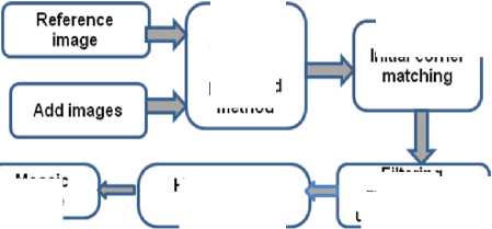
Mosaic image

Homography estimation

Filtering mismatches using RANSAC

Figure 1. Mosaic image flow

This paper is organized as follows: In section I, the process of image stitching is explained in detail. In section II, the basics of various feature point detectors are briefly described. The feature descriptors extraction and matching are briefly described in sections III and IV. The feature point and mosaic results are presented in section V. Finally, this paper is concluded in section VI.

• II.    FEATURE POINT DETECTION

• A.    Harris Corner Detector

Harris detection algorithm is based on the assumption that corners are associated with maxima of the local autocorrelation function. Calculate the change of pixel gradient. If the absolute gradient value changes significant in all directions, then declare the pixel as a corner.

R= det(M)- k(trace(M))2			(1)
	Vs / 1 2	9 1 9 1
M=G(σ)*	Id x )	9 x 9 y	(2)
	9 I 9 I	2 f az1
	9 x 9 y	l9 y ) _

R is measure the corner response at each pixel coordinates ( x, y ). k is a constant and typical value is 0.04. ⁹ I , ⁹ I represents the first order gray gradient of

9x dy horizontal and vertical, G(σ) is an isotropic Gaussian filter with standard deviation σ and the operator * denotes convolution.

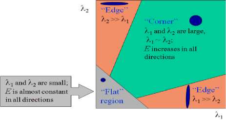
Figure 2. Harris operator

In figure 2. ^, ^ is proportional to the principal curvatures of partial autocorrelation function. There, by judging the values of ^ and ^ to determine the slow change corner and edges. As per the gradient changes shown in fig 2, are three cases[4] when the two curvatures are low this shows that local autocorrelation function is very flat, changes are not dramatic; If one curvature is low and the other is high, this means partial autocorrelation function changes in one direction means it’s edge. When the two curvatures are high, indicating the local autocorrelation function has a peak, it’s the corner. This is a fast and simple detector and is less sensitive to noise in image than most other algorithms, because the computations are based entirely on first derivatives.

• B.    KLT (Kanade-Lucas-Tomasi) Corner Detector

The KLT corner detector [7] has two parameters: the threshold on ^ , denoted by Д ^, and the linear size of a square window (neighbourhood) D X D.

The KLT Corner Detector algorithm:

• 1.    Compute C at each point ( x, y ) of the image.

• 2.    For each image point p =( x, y )

(a)Find the smallest value of ^ in D-neighborhood of p .

• (b) If that ^ >  Д ^, save p ( x, y ) into a potential list L .

• 3.    Sort L in decreasing order of ^

• 4.    Scan the sorted list from top to bottom. For each current point p , delete all lower points in the list in the

D-neighborhood of p .

The KLT algorithm produces a list of feature points that have ^ >  ^_th and the neighborhood D of these points do not overlap. The parameter selection A_thr may be estimated from a histogram of ^ : usually A_thr is selected as a valley of the histogram. Window size D is usually between 2 and 10, select by trial and error. For large D the corners may move away from the actual position and some close neighbour corners may be lost. This detector uses explicit calculation of Eigen value ^ and produces good repeatability.

• C.    FAST ( Features from Accelerated Segment Test ) Corner Detector

Fast corner detector [7,8] based on segment test. Consider a sixteen pixels circle around the point p as shown in fig 3. The p detected as a corner if there exists a set of n contiguous pixels in the circle which are all brighter than the intensity of the candidate pixel Ip+t , ( t- threshold) or all darker than Ip-t, as shown in fig 3. n was originally chosen to be twelve because it admits a high-speed test. The test examines only the four pixels at 1, 5, 9 and 13, that are four compass directions. If p is a corner then at least three of these must all be brighter than Ip + t or darker than Ip - t. If neither of these is the case, then p cannot be a corner. Segment test can be applied to the remaining candidates by examining all pixels in the circle. This detector exhibits high performance and it is fast. In this paper we use n=9, which is the most reliable of the FAST detectors.

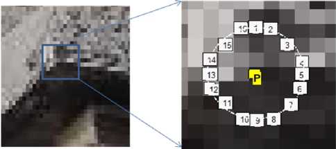
Figure 3. Segment point detection in a image patch. The pixel at p is the centre of a candidate corner.

• D.    Steerable filters

Steerable filters, introduced by Freeman and Adelson[9,10] are spatial oriented filters that can be expressed using linear combinations of a fixed set of basis filters. If the transformation is a translation, then the filter is said to be shift able or steerable in position; if the transformation is a rotation, then the filter is said to be steerable in orientation or commonly steerable and the basis filters are normally called steerable basis filters. Given a set of steerable basis filters, we can apply them to an image and since convolution is linear, we can interpolate exactly, from the responses of the basis filters, the output of a filter tuned to any orientation we desire. Steerable filters are describing a class of filters in which a filter of arbitrary orientation is synthesized as a linear combination of set of “basis filters”.

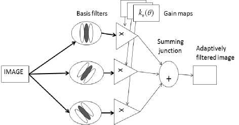
Figure 4. Steerable filter block diagram

The basic idea is to generate a rotated filter from a linear combination of a fixed set of basis filters. Fig 4 shows a general architecture for steerable filters, which consists of a bank of permanent, dedicated basis filters that always convolve the image as it comes in. The outputs are multiplied by a set of gain masks, which apply the appropriate interpolation functions at each position and time. The final summation produces the adaptively filtered image. The steerability condition is not restricted to derivative filters and could be expressed for any signal f as:

M fθ(x,y)=∑km(θ)fθm(x,y)                  (3)

m = 1

where f ^θ ( x , y ) is the rotated version of f by an arbitrary angle 9 , k m (9) are the interpolation functions, f ^{θ m} ( x , y ) are the basis functions and M the number of basis functions required to steer the function f ( x , y ) .

To determine the conditions under which a given function satisfies the steering condition in (3), let us work in polar coordinates ( _{r = x} ² ₊ y ² and φ = arg (x,y)) .

The function f could be expressed as Fourier series in polar angle φ :

N

f ( r , φ ) = ∑ a n ( r ) e^{jn φ}                        (4)

n=-N where j= -1 and N is the discrete length of coefficients. It has been demonstrated in [9] that the steering condition in (3) is satisfied for functions expandable in the form of (4) if and if only the interpolation function km(9) are solution of:

M cn(θ) = ∑km(θ)(cn(θ))m                   (5)

m =- 1

where c n = e ^{jn θ} , and n ={0,…, N }.

From (5), f ^θ ( r , φ ) is expressed as:

M f θ(r,φ) = ∑km(θ)gm(r,φ)                  (6)

m = 1

where g ( r , φ ) can be any set of functions.

It has been also demonstrated that the minimum number M of basis functions required fto( rst,eφe)r is equal to the number of non-zero Fourier coefficients an(r).

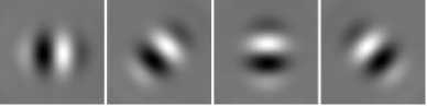
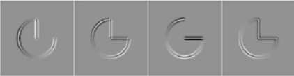
Figure 5(a) original image applied to the basis filters of the steerable filters are directional derivative operators with four orientations 00,450,900 and 1350 representation as shown in fig.5(b), figure 5(c) shows the output images at different orientations.

(a)

(b)

(c)

Figure 5.  (a) original image (b) four oriented 00,450,900 and 1350

basis filters (c) output images

• E.    Proposed Corner Detection

We propose new corner detection using the steerable filters[9] and Harris algorithm as follows:

• 1.    Decomposition of an image with different orientations using steerable filters

• 2.    Detect the corners in each direction using Harris algorithm.

• 3.    Combine all detected corners by performing logical or operation.

• 4.    Applying dilation to the combined nearby corners to make them into one.

• 5.    Find the centroid of step 4 and identified as corner.

We propose a corner detection algorithm as shown in fig 6. that uses the steerable filters. The experiments carried out with matlab make it clear that if the number of orientations is four, it gives better localization and minimum number of false corners detection.

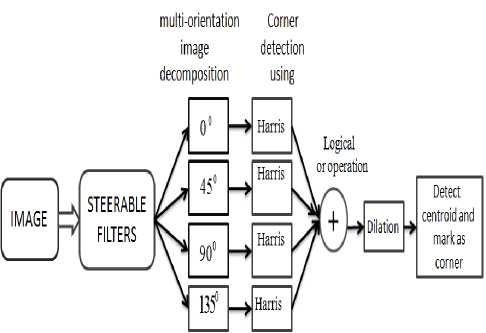
Figure 6. Proposed algorithm

• III.    FEATURE DESCRIPTOR EXTRACTION

Here the local feature points are detected using Harris corner detectors in each image. Each of the feature points is given an "identity". Without the "identity", the feature points are just purely coordinators that indicate where the features are located, and the feature points cannot be matched. Hence, a feature point descriptor is required to generate an "identity" for each of them. So, extract feature descriptor for each feature point. Descriptors are simple a 21x21 gray scale pixel patches extracted from an image blurred by a Gaussian (sigma=3 pixels). The blurring is done to obtain some tolerance to feature localization errors; a 21x21 feature point descriptor is used in this paper. The "identity" will be usually generated using the information that is obtained from the neighbouring pixels of a feature point.

• IV.    FEATURE MATCHING

In this step, the correspondence between feature points, P , in the reference image and feature points, P’ , in the input image are evaluated. The best candidate match for each feature point is found by identifying its nearest neighbour in the data set of feature vectors from input image. The nearest neighbour is defined as the feature point with minimum Euclidean distance for the invariant descriptor vector.

• A.    Homography Estimation using RANSAC

Random Sampling Consensus (RANSAC)[11] is an algorithm to fit a model to the data set while classifying the data as inliers and outliers. This algorithm has been applied in estimating the fundamental matrix to match two images with wide or short baseline and estimating a homography. A set of inliers can be determined from an input data set of points. It proceeds as follows:

• 1.    Sample N times from the data set randomly. N is the number of trials required to achieve a confidence level p , which is chosen around 0.9 ~ 0.99

• 2.    Select 4 pairs of sample points and make sure that no three of them are on the same line. Compute H through the sample points.

• 3.    Compute the distance between the matched inliers after the H transformation.

• 4.    Compare the distance with the threshold. If it is less than the threshold, keep the points as inliers. Compute the H from the sub-data-set which contains the most inliers.

• B.    Image mosaics

After computing the transformation function for each image, we can compose images into one big image. If we stitch the images directly, the blending image will contain obvious boundaries due to the luminance difference. The fade-in and fade-out method can be implemented to reduce the stitched images gap. The value of the pixel in the overlapping image is weighted as average value of the corresponding pixel in the two images.

• V.    EXPERIMENTAL RESULTS

The performance of feature detectors can be expressed in terms of repeatability[12,13]. The good feature detectors should have a high repeatability rate (good stability). We compute the repeatability rate that evaluates the geometric stability of points under different image transformation.

A. Repeatability

The repeatability rate for a given pair of images is computed with the ratio between the number of point-to-point correspondences and the number of possible corresponding detected in the images. We take into account only the points located in the part of the scene present in both images. We use test images with homographies to find the corresponding regions.

Repeatability rate= # correspondences (7) # possible correspondences

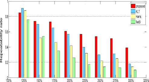
First, an experiment is conducted with original Ellora caves image and its transferred image. The transferred image obtained with a scale change in steps of 25% variations between 125% and 300% is as shown in Fig 7(a).

Scale factor

(a)

(b)

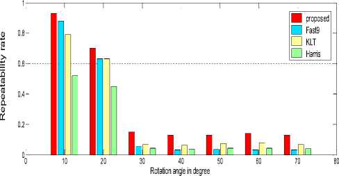
Figure 7. Repeatability rate: (a) scale change and (b) rotation

It is observed that the KLT gives good performance and is indicated with blue colour. The proposed method gives still better performance indicated with red colour and observed between 150% and 300% compared with the other detectors.

Fig. 7(b) shows repeatability for image rotation. The rotation angles vary between 0 to 70 degrees in steps of 10 degree. It is observed that the detectors are very sensitive to rotation changes. The Fast9 gives good performance and indicated with blue colour. Our method which is indicated in red colour gives still better performance. The proposed method uses steerable filters that contain banks of fixed basis filters that enhance the corner stability. In this paper, image mosaic is implemented using proposed method.

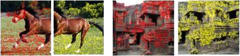
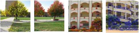
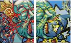
Feature point detection and mosaic experiments conducted and tested on different number of various image pairs are shown in Fig 8.

(a)                                      (b)

(d)

(e)

Figure 8. Test image pairs (a) Horse (b) Ellora caves (c) Tree (d) Building (e) Graffiti (f) Satellite image.

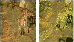
(f)

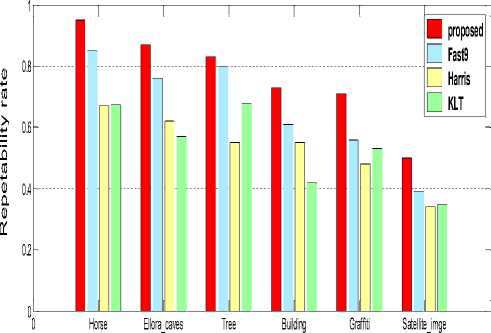
Figure 9. Repeatability rate for different image pairs

Fig 9. shows the repeatability rate[14] for different images for mosaic results. Our method performs better repeatability than other methods.

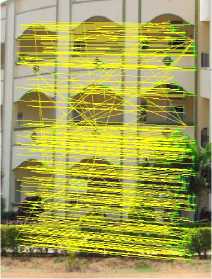
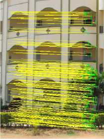
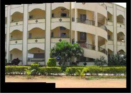
The mosaic experiments are carried out and tested number of images with different sizes. It can be concluded that the matching results obtained are accurate and stable. The detected features are 1465 and 1825 in the two input images used for stitching. Fig.10 (a) shows 271 initial matches found. Fig. 10(b) shows 199 correct matches using proposed method. Fig.10(c) shows the mosaic image.

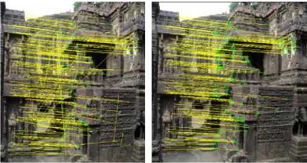
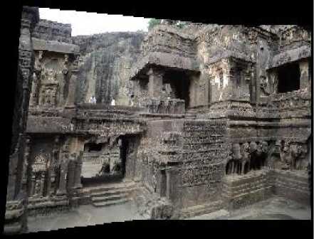
Fig.11 shows another mosaic process of two Ellora Caves images, with sizes of 512 x512 to be stitched. Fig.11(a) and 11(b), shows 206 initial matches and 180 correct matches respectively using proposed method. Fig.11(c) shows the of mosaic image.

(a)                                (b)

(a)                                   (b)

(c)

Figure 10. (a)-(c) Building image Mosaic results using feature points

(c)

Figure 11. (a)-(c). Ellora caves image Mosaic results using feature Points

TABLE 1. IMAGE MOSAIC RESULTS

Methods	Image size	Number of corners detected	Number of initial matches	Number of correct matches	Repeata bility rate %	Time in sec
KLT	Fig10(a) 360x440 Fig10(b) 360x440	184 354	89	38	42.69	1.490
Harris		313 336	134	74	55.22	1.618
Fast_9		769 811	322	199	61.80	1.265
Proposed		1465 1825	271	199	73.43	1.817
KLT	Fig11(a) 512x512 Fig11(b) 512X512	666 799	162	92	56.79	1.458
Harris		908 1066	340	210	61.7	1.597
Fast_9		2641 3112	743	566	76.17	1.38
Proposed		3120 3031	206	180	87.4	2.156

The numbers of corner points detected, initial match numbers, correct matches and repeatability rate as shown in table 1. It is observed that the proposed method has better repeatability rate. So it can be concluded that proposed method is effective compared to other detectors.

• VI.    CONCLUSION

In this paper, the performance of various feature point detectors extracting feature points is shown. It can be seen that success rate of stitching is strongly related to number of feature points. However, it is not wise to blindly increase the number of feature points that can be extracted by a detector, since it will lead to increase in processing time due to massive amount of matching operation.