Fixed Windows in Fractional Fourier Domain

Published Online January 2014 in MECS DOI: 10.5815/ijigsp.2014.02.01

Several applications of window functions have been reported in the fields of signal processing and communications, such as digital filter design, spectrum estimation, beam-forming, and speech processing [1]. The useful parameters of window functions for these applications include Half Main Lobe Width (HMLW), Normalized Band Width (NBW), Maximum Side Lobe Level (MSLL), and Side Lobe Fall of Rate (SLFOR). A concise analysis of these parameters and their properties has been presented by Harris [2]. In [2], Harris has described time domain and frequency domain parameters of window functions. Frequency domain behavior of window functions has been studied by mapping the time domain window function in frequency domain using Fourier Transform (FT).

In this study, characterization of window function parameter has been carried out in fractional Fourier domain which is a generalization of the FT. The Fractional Fourier Transform (FRFT) with an additional adjustable parameter, FRFT order ( a ), makes it more flexible and is having numerous applications in many areas [3-5], where as its implementation cost is at par with FT.

The continuous-time FRFT of a signal x (t) is given as [5]- то

X_a ( u ) = J x ( t ) K_a ( t, u ) dt     (1)

—TO where, the transformation kernel Kα (t, u) of the FRFT is defined as-

^{2  2} ^

— M ^а j - rntcosec ( « )

-------------e V if а Ф nn if а = 2nn

У    2 n

^K « ( t , ^u ) = <

5 ( t — u )

5 (t+u)                     if (а+n) = 2nn where, α = aπ / 2 is the rotation angle of the transformed signal of the FRFT.

Prior to this work, analysis of some window functions in FRFT domain has been carried out by Kumar et al. [6], and it has been observed that the window parameters can be varied by changing the FRFT order. However, no mathematical relationships have been established between window parameters and FRFT order in [6] . It has been shown in [6] that when FRFT order is decreased from 1 to 0, the MSLL and SLFOR increase while HMLW decreases. Same methodology has been used earlier in [7] to tune the Transition Bandwidth (TBW) of Kaiser Window [2] and PC6 window [8] based FIR filters using FRFT. It has been shown in [7] that when the FRFT parameter is decreased the Transition Bandwidth (TBW) of the window based FIR filter decreases. Variations in the better TBW have been obtained without re-computation of filter impulse response coefficients. However, the applicability of this phenomenon has been demonstrated in [7] only for lower order FIR filters.

In this paper, analysis of rectangular (Dirichlet), generalized 2 -term cosine (Hanning / raised cosine / Hamming), Blackman and triangular window functions in FRFT domain has been reported. These windows fall in the fixed windows category. Relationships between window function parameters and FRFT order have been established. These relationships have been utilized in the design of fixed window based FIR filters.

The rest of paper is organized as follows: In Section-2 characterization of windows in FRFT domain has been carried out. Limiting values for the length of window functions, about which their NBW shrinks and expands, have been determined in Section-3. This analysis is based on the principle of uncertainty product for the window function [9]. The relationships established in previous sections have been used in Section-4 for the designing of FIR filters. Finally, the paper is concluded in Section-5.

I WR ( U ),

1 - icot ( a )

-

II. CHARACTERIZATION OF WINDOW FUNCTIONS IN FRACTIONAL DOMAIN

The mathematical analysis of fixed windows in the FRFT domain has been carried out in this section to establish the relationships between window parameters and FRFT order. Plot shown in Figure 1 illustrate the four frequency domain parameters for a window function, viz. MSLL, SLFOR, HMLW, and NBW, for which the relationships in fractional Fourier domain have been established. Characterization has been carried out for four fixed windows- (a) Rectangular (b) Generalized Hamming (c) Blackman (d) Triangular window, as given in following section-

The mathematical relationships for NBW, MSLL, and HMLW in fractional domain have been obtained by differentiating the fractional domain response of the window functions. This follows from the mathematical

results that the position of maxima and minima of any function can be obtained by the differentiation of that function.

The plots for the magnitude of W R ( u ) and its

differentiation with respect to u for α = 0.4 are shown in

Figure 2 and 3 respectively. From these figures it

follows that the zeros of

dl ^{( u} )

occur at the

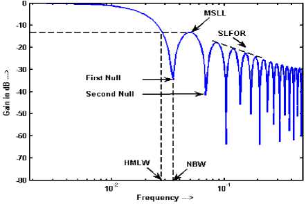
Figure 1. Plot for illustrating the definition of the parameters of window function

positions similar to the null positions of | W R ( u )|. Thus, the position of the window’s FRFT nulls can be obtained by differentiating (4) with respect to u and equating it to zero as given in Appendix-2

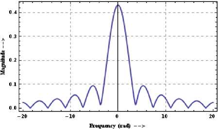
Figure 2. FRFT of rectangular window for τ = 1 and a = 0.4

A. Rectangular Window (RW)

The time domain expression for a RW is given as-

wR ( t ) = *

1,

t <  -

The FRFT domain expression W_R ( u ) of RW (A1.4) has been included in Appendix-1.

The magnitude of W R ( u ) for this window is given by-

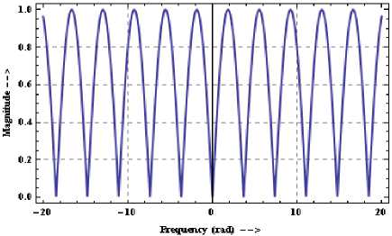
Figure 3. Plot for the differentiation of | W_α(u) | with respect to u

The position of nulls of | W_R ( u )| for various values of n are given by (A2.6) and for n = 1 it determines the

TABLE I. DISCRETE RW PARAMETERS FOR N = 25 AND M = 2048

FRFT Order, a	NBW		HMLW		MSLL (dB)
	SR	AR	SR	AR	SR	AR
1.0	0.04	0.04	0.0323	0.0324	-13.23	-13.2627
0.9	0.0396	0.0395	0.0320	0.0320	-13.21	-13.2618
0.8	0.0381	0.038	0.0310	0.0300	-13.20	-13.2591
0.7	0.0357	0.0356	0.0290	0.0289	-13.19	-13.2540
0.6	0.0323	0.0324	0.0263	0.0262	-13.15	-13.2450
0.5	0.0284	0.0283	0.0230	0.0229	-13.10	-13.2293
0.4	0.0236	0.0235	0.0200	0.0190	-13.01	-13.1997
0.3	0.0183	0.0182	0.0150	0.0147	-12.79	-13.1355
0.2	0.0120	0.0124	0.0110	0.0100	-12.20	-12.955
0.1	0.0060	0.0063	0.0052	0.0051	-9.380	-12.070

NBW of the RW. Thus, the NBW in FRFT domain for RW ( u NR ) is –

uNR

The coefficient of sin ( α ) in the above expression defines the NBW of continuous time RW in Fourier domain. On the other hand, for N -point discrete time RW the transition width of mainlobe in FT domain is given by 4π/ N [10] which can be normalized to define NBW as 1/ N .

Thus, the above relation expresses u NR in terms of NBW in Fourier domain, i.e., u FT as-

The magnitude of MSLL has been obtained by substituting (7) in (4) as given by (8)-

U nr = U ^TT sin ( a )|         (6)

MSLL_R

where,

1 - icot ( a )

2 n

u FT

,

т

I N ’

for continuous - time RW for discrete - time RW of N samples

erfi +i^ ^ cot ( a ) { 0.5 т - 1.425 u_FT tan ( a

-

■ erfi ^-+ ⁱ ^ c ot ( a ) { - 0.5 т - 1.425 u_{F r}tan ( a

It has been observed from the simulation studies that the MSLL occurs at 1.425 times of NBW as shown in Figure 4 ( shown from 0 to 0.2 in place of actual range 0 to 0.5 for the sake of clarity ). Therefore, the expression for the position of MSLL of RW can be written as-

It has been shown in [11, 12] that HMLW of RW is 0.81 times of NBW. Therefore, the HMLW in FRFT domain, u_HR , can be expressed as-

UHR

|0.81 U f_t sin ( a )|

U mr = |1.425 u ft sin ( a )|         (7)

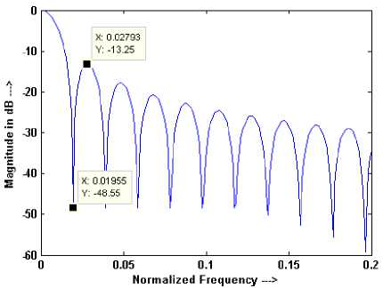
Figure 4. Plot for the position of NBW and MSLL of RW for window length N = 51

The obtained Analytical Results (AR) for NBW, MSLL and HMLW has been verified using Simulation Results (SR). The recorded values for these parameters are shown in Tables I.

The expressions for other fixed windows have been also obtained in FRFT domain by following the same methodology adopted in RW.

B. Generalized Hamming Window (GHW) The GHW is defined in time domain as-

wH ( t ) =

b + ( 1 - b ) cos ( 2 nt ) ,    |t | <  0.5

0,                   elsewhere

For b = 0.5, Hanning window results while for b = 0.54, Hamming window results.

TABLE II. DISCRETE HW PARAMETERS FOR N = 35 AND M = 2048

FRFT Order, a	NBW		HMLW		MSLL (dB)
	SR	AR	SR	AR	SR	AR
1.0	0.0590	0.0571	0.055	0.0534	-31.47	-31.4743
0.9	0.0581	0.0564	0.054	0.0528	-31.44	-31.4717
0.8	0.0562	0.0543	0.052	0.0500	-31.35	-31.4635
0.7	0.0528	0.0500	0.048	0.0476	-31.16	-31.4478
0.6	0.0480	0.0462	0.045	0.0432	-30.85	-31.4206
0.5	0.0422	0.0400	0.039	0.0378	-30.29	-31.3731
0.4 *	0.0350	0.0336	0.029	0.0310	-29.18	-31.2843
*Unable to observe

The fractional domain expression of the GHW (A3.1) has been obtained by following the similar steps of RW and given in Appendix-3.

Since the NBW of GHW ( u NH ) is twice that of NBW of RW ( u RH ) [10, 13]. Therefore, using (6) u NH can be expressed as-

The expression for the MSLL in FRFT domain of GHW with b = 0.5 has been obtained by substituting (12) in (A3.1) and given by (A3.2).

It has been shown in [11, 12] that the HMLW is at the 0.935 and 0.955 times of NBW for b = 0.5 and 0.54 respectively. Therefore, it can be expressed in FRFT domain as- uNH   u^TT sin (^% )|

where,

u

'| 0.935 u

^HH   [|0.955 u

FT

FT

sin ( a )| sin ( a )|

when b = 0.5

when b = 0.54

4 n

u FT ⁴

T

I N ,

for continuous - time GHW for discrete - time GHW of N samples

The obtained expressions for NBW, MSLL and HMLW of GHW have been verified with simulation studies. The recorded values for Hanning Window (HW) are shown in Tables II.

It has been observed that the MSLL of GHW occurs at the 1.175 and 2.135 times of NBW for b = 0.5 and 0.54 respectively as shown in Figure 5. Thus, it can be written as-

C. Blackman Window (BW)

The expression for the BW in time domain is given as-

u_MH

11.175 u_FT sin (a )|

2.135 u  sin ( a )|

when b = 0.5

when b = 0.54

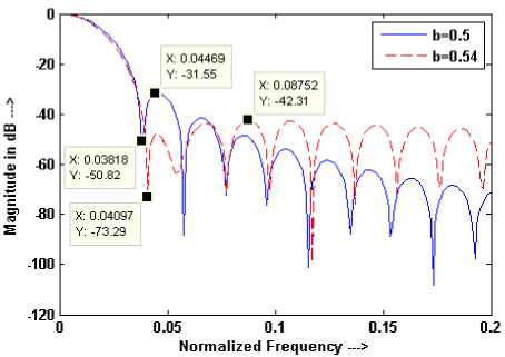
Figure 5. Plot for the position of NBW and MSLL of GHW for window length N = 51

w_B

(t ) =

0.42 + 0.5 cos ( 2 n t ) + 0.08 cos(4 n t ), | t | <  0.5

0,                              elsewhere

The expression for the BW (A4.1) in FRFT domain is given in Appendix-4.

Since the NBW of BW ( u NB ) is thrice that of NBW of RW ( u RH ) [10, 13]. Therefore, using (6) u NB can be expressed as-

UNB

where,

u F'T

u sin

FT

6n

2 . N ’

for continuous - time BW for discrete - time BW of N samples

It has been observed that the position of MSLL of BW is 1.18 times of NBW as shown in Figure 6. Thus, it can be defined in FRFT domain as-

u MB

11.1 8u_FT sin ( a )|

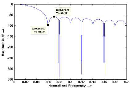
Figure 6. Plot for the position of NBW and MSLL of BW for window length N = 51

The FRFT domain relationship for the MSLL of BW (A4.2) has been obtained by substituting (16) in (A4.1) and given in Appendix-4.

The position of HMLW for BW [11, 12] in FRFT domain can be written as-

UHB

1 0.94u_FT sin ( a )|

The obtained expressions for NBW, MSLL and HMLW of BW have been verified with simulation results and recorded values are included in Tables III.

TABLE III. DISCRETE TW PARAMETERS FOR N = 35, M = 1024

FRFT Order, a	NBW		HMLW		MSLL (dB)
	SR	AR	SR	AR	SR	AR
1.0	0.0590	0.0571	0.0480	0.0465	-26.32	-26.5325
0.9	0.0576	0.0564	0.0473	0.0459	-26.32	-26.5323
0.8	0.0552	0.0543	0.0453	0.0442	-26.33	-26.5353
0.7	0.0514	0.0509	0.0431	0.0414	-26.36	-26.5351
0.6	0.0473	0.0462	0.0396	0.0376	-26.46	-26.5383
0.5	0.0421	0.0404	0.0358	0.0329	-26.45	-26.5439
0.4	0.0359	0.0336	0.0315	0.0273	-26.56	-26.5545
0.3	0.0307	0.0259	0.0261	0.0211	-26.80	-26.5777
0.2 *	0.0229	0.0177	0.0198	0.0144	-27.38	-26.6443
*Unable to observe

TABLE IV. DISCRETE BW PARAMETERS FOR N = 45 AND M = 1024

FRFT Order, a	NBW		HMLW		MSLL (dB)
	SR	AR	SR	AR	SR	AR
1.0	0.0683	0.0667	0.0641	0.0627	-58.12	-58.1115
0.9	0.0702	0.0658	0.0642	0.0619	-58.14	-58.1124
0.8	0.0688	0.0634	0.0644	0.0596	-58.21	-58.1155
0.7	0.0655	0.0594	0.0624	0.0558	-58.27	-58.1212
0.6	0.0602	0.0539	0.0575	0.0507	-58.19	-58.1311
0.5 *	0.0471	0.0530	0.0443	0.0514	-57.45	-58.1480
*Unable to observe

D. Triangular Window (TW)

The expression for the TW in time domain is given as-

Since the NBW of TW (uNT) is twice that of NBW of RW (uRH) [10, 13]. Therefore, using (6) uNT can be expressed as- uNт= Ц-рt sin (a)| (19)

w

(t )=

1 - 2 t l, *        T

where,

elsewhere

The FRFT domain expression of TW (A5.1) is given in Appendix-5.

u_FT

4n

' 2

. N ’

for continuous - time window for discrete - time TW of N samples

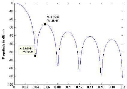
Again, it has been observed by the simulation studies that the position of MSLL of this window is 1.45 times of NBW as shown in Figure 7. Therefore, it can be defined in FRFT domain as- uMT

1 145u_FT sin ( a )|

The fractional domain expression for the MSLL of TW has been obtained by substituting (20) in (A5.1) and is given by (A5.2) as shown in Appendix-5.

The position of HMLW of TW [11, 12] can be written as- инт = |0.815uFт sin (a)|

this particular window length in FRFT domain. It has been observed in simulation studies that the NBW shrinks for small window length and expands for large window length when the FRFT order is varied from 1 to zero because frequency plane moves toward time plane i.e. window length. Thus, the FRFT provides another parameter to vary the NBW without varying the window length.

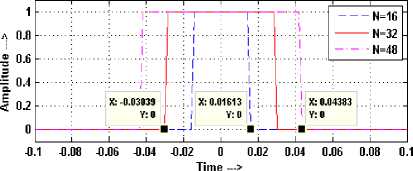
It has been observed by simulation studies that the time spread of M zero padded discrete windows of length N equals to the main lobe width of window function at particular window length (limiting length, N ) for a = 1. To find this limiting length N , time domain and frequency domain spread of RW has been shown in Figure 8.

The derived expressions for NBW, MSLL and HMLW of have been verified with simulation results. The recorded values are included in Tables IV.

Normalized frequency —>

Figure 7. Plot for the position of NBW and MSLL of TW for window length N = 51

(a)

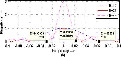
Figure 8. Expanded view of RW (a) time domain (b) frequency domain for different length N and M = 512 with a = 1

• III.    UNCERTAINTY PRODUCT IN FRACTIONAL DOMAIN

It is easy to verify from that the FRFT holds an identity operator i.e. signal attains fully time domain behavior for a = 0 while it is conventional FT i.e. signal jumps into frequency domain completely for a = 1. If the FRFT order a lies between these two ranges signal will be composed of frequency and time components both. In FT domain, the NBW is having inverse relationship to the window length and the product of these two parameters remains constant for every window function. This property of window functions can be thought of as the uncertainty principle [9] according to which a function in time domain and its FT cannot both be highly concentrated. If the window length is small the NBW is large and at particular window length these two parameters become equal and further increment from this window length NBW becomes smaller than the window length. This property of window functions has been exploited in this work to analyze the behavior of windows for below and above of

The x-axis of both the domains of N sampled and M zero padded RW has been normalized in the same range i.e. -0.5 to 0.5 however, it has been shown only in the range of -0.1 to 0.1 for the sake of clarity. The non-zero time spread of the normalized window is given by ( N +1)/( M + N ) and N /( M + N ) for N is odd and even respectively. The range of main lobe width of RW in the normalized frequency domain spread is given by -1/ N to 1/ N . Thus, the generalized expression of the limiting length of fixed windows at which half width of the window function in time domain equals to the NBW in frequency domain can be obtained for above reported window functions from (6), (11), (15), (19) respectively at a = n/2 as-

N + 1   _ p

2 ( M + N ) = N

if N is odd

N p

—-------- = — if N is even     (22)

The mathematical relation given in (22) is a quadratic equation and its positive root, which defines the limiting length of window functions, is given as-

N = p +

P +

2 M

^p

The value of N given by (23) is the limiting length of the fixed window functions above which the NBW expands by decreasing the value of FRFT order a from 1 to zero. The obtained limiting length for RW ( p = 1) with padded zeroes M = 512 is N = 32 at which NBW and half width of RW becomes equal as shown in Figure 8. It can be also observed from Figures. 9-10 that the NBW of RW reduces by decreasing the value of a from 1 to zero if the number of samples in the window are less than 32 and expands if the samples are more than 32 Similar behavior has been also observed for other fixed windows as shown in Figures.11-16. Figures 9-16 have been shown from 0 to 8 bins only in place of actual range 0 to N /2 bins for the sake of more clarity.

Figure 11. Frequency response of HW with a for N = 43 and

M = 512

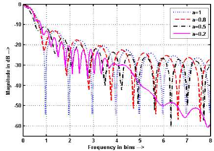
Figure 9. Frequency response of RW with a for N = 27 and M = 512.

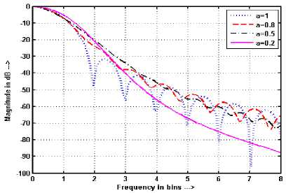
Figure 12. Frequency response of HW with a for N = 53 and

M = 512

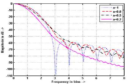
Figure 13. Frequency response of BW with a for N = 70 and M = 1024

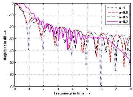
Figure 10. Frequency response of RW with a for N = 37 and M = 512

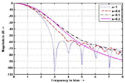
Figure 14. Frequency response of BW with a for N = 90 and M = 1024

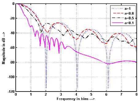
Figure 15. Frequency response of BW with a for N = 39 and

M = 512

Filtered Output

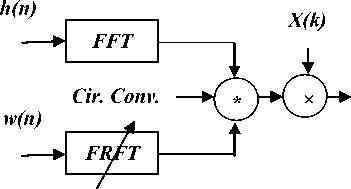
Figure 17. Tuning scheme of FIR filters using FRFT

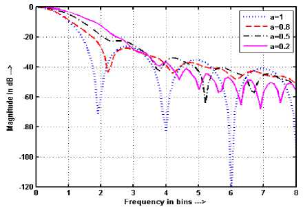
Figure 16. Frequency response of BW with a for N = 57 and M = 512

The tuning of frequency responses of FIR filters using Hanning and Blackman windows are shown in Figures. 18-21. It has been observed from these responses that, by varying FRFT order from 1 to 0, the TBW of FIR filters decreases according to f_c + u_FT sin ( α ) approximately, where f_c is the cutoff frequency of the filter, and SBA and PBR increases if the filter order is less than (23) while behavior of these parameters becomes opposite if the order of filter is greater than (23). Theoretically, this happens because if the length of window is equal to (23) then the window spans in time domain and frequency domain are equal at FRFT order 1 while time span becomes less than frequency span and tends toward impulse function if the length of window is less than (23) when FRFT order decreases from 1 to 0 and it becomes vice versa for the window length greater than (23). This behavior of window functions is directly affecting parameters of FIR filters designed using these fixed window functions. Thus it can be said that parameters of windowed FIR filters can be tuned using FRFT up to the filter designed without windowing i. e. impulse response method without re-computing the filter coefficients.

• IV.    TUNING OF FIR FILTERS

The TBW of window based FIR filters is proportional to the filter order. Thus, it can be varied by the variation of filter order which needs the re-computation of the impulse response coefficients of the filter. An alternative FRFT based method to tune the TBW of these filters using ideal impulse response has been developed by Sharma et al. [7] which eliminates the recomputation problem. In this work, in place of ideal impulse response of the filter, realistic impulse response h(n) has been used and characteristics of FIR filter i. e. TBW, Stopband Attenuation (SBA) and Passband Ripple (PBR) are being varied by varying the frequency response of window function w(n) with the variation of FRFT order a . To obtain the filtered output in frequency domain the circularly convolved output of FFT of impulse response h(n) i.e. H(k) and FRFT of w(n) is multiplied by FFT of input signal x(n) i.e. X(k) as shown in Figure 17 .

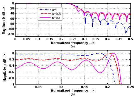
Figure 18. Frequency responses of LPF using HW with fp = 0.2, fs = 0.3, N = 31 (a) Comparative frequency responses (b) expanded view of passband

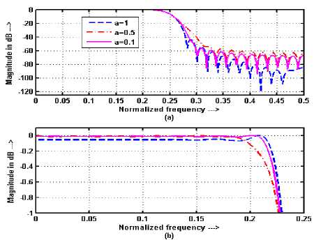
Figure 19. Frequency responses of LPF using HW with fp = 0.2, fs = 0.3, N = 51 (a) Comparative frequency responses (b) expanded view of passband

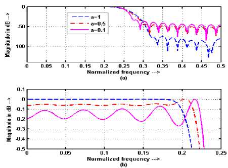
Figure 20. Frequency responses of LPF using BW with fp = 0.2, fs = 0.3, N = 41 (a) Comparative frequency responses (b) expanded view of passband

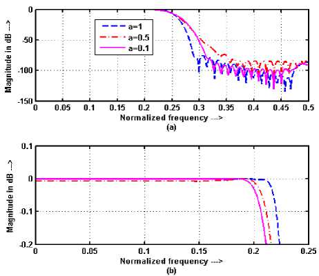
Figure 21. Frequency responses of LPF using BW with fp = 0.2, fs = 0.3, N = 71 (a) Comparative frequency responses (b) expanded view of passband

• V.    CONCLUSION

The analytical expressions have been derived for four popular fixed window functions. It has been observed that the window parameters like NBW, HMLW and MSLL may have one more controlling variable (FRFT order a ). The derived expressions have been verified with simulation studies in all situations. Thus, it can be said that these windows can be considered as variable windows in time-frequency plane, keeping their time domain nature unchanged, which are inherently fixed in nature. The derived expressions can be considered very useful in more efficient design of window based digital FIR filters and spectral analysis. The obtained adaptability in the fixed windows has been exploited in the tuning of the parameters of FIR filters.