Focal-plane field when lighting double-ring phase elements

One of the simplest diffractive optical elements (DOE) is a circular plate with thickness step corresponding to phase difference of 180 degrees. Despite its design simplicity, this element happens to have several practical applications.

In particular, such plates are used to align intensity of focused Gaussian beams [1]. Moreover, we mean not to focus on a ring/square, but somewhat differently – to obtain a domain with dimensions close to diffraction limits with approximately uniform intensity (not necessarily with sharp edges). DOE proposed in paper [1] in the form of a ring or square step is the simplest element among all considered elements used to solve similar problems [2–4]. In paper [5], two stepped elements are used for onedimensional dynamic beam correction.

Another application for phase-step plates is sharp focusing. Phase steps are used in accordance with the first Hermite-Gaussian mode to excite an electric-field longitudinal component at the focus center; this was considered in papers [6–8]. It is shown in papers [9, 10] that a focal pattern and, accordingly, contribution of the longitudinal component to the central part of focal domain is influenced by mutual arrangement of polarization axis and a phase step curve for the plate. Besides, in paper [11], the phase-step plate is used to study polarization sensitivity of a near-field microscope.

Radial-step phase plates are also used for sharp focusing and in polarization transformations [12]. In this case, they are capable to perform similar functions like either of multi-ring or multi-level phase plates [13– 16]. Iterative or other optimization algorithms are often used to calculate them. The advantage of simple elements (binary one- or two-ring) lies in their ability to analytically evaluate their activity [17, 18].

Sharp focusing of radial-polarized beams is considered in paper [17]. Interrelation between width of a diaphragm ring with the introduced radial phase step and focal spot dimensions and intensity values is also studied there. It is shown that due to destructive interference generated by rings with different phases, it is possible to skip scalar limits related to the first zero of the zero-order Bessel function. The minimum focal spot size (FWHM=0.33λ) is achieved when diaphragm ring width is 20 per cent of radius of a full aperture. In this case, intensity of side lobes does not exceed 30 per cent of a central peak. It is also shown that by introducing phase steps and simultaneously widening a ring aperture, it is possible to generate the focal spot not exceeding the size limit corresponding to a narrow ring aperture while intensity increases almost 6 times. Furthermore, side lobes embrace 35 per cent of the central peak.

Paper [18] cites evidence that two annular zones are sufficient for many problems. Analytical estimates are obtained for parameters of a two-zone element in off-axis scalar approximation; the element provides maximum values of interference maxima on optical axis. Zone radii coincided with zone-plate radii. However, a zone plate with free-space limiting numerical aperture has its central zone r 1 = 1.12 λ in radius, and remaining zones are represented by rings less than λ /2 wide. In this case, decaying waves get mostly through a peripheral part of the optical element; they slightly affect distribution near optical axis. Therefore, it is possible to discuss influence of only one or two central zones. It is shown numerically and analytically that an optical microelement, consisting of only two axially aligned annular zones, can be used for sharp focusing of laser radiation. Moreover, the greatest focusing degree is achieved when the central zone is λ /2 in radius.

Here, as in paper [18], influence of the total element (instead of the ring element) is regarded in far-field diffraction. Though a more accurate off-axis model is used in paper [18], analytical calculation was carried out only for the optical axis field. The transverse in-plane field corresponding to the lens focal plane is analyzed in this paper.

1.    Theoretical study of double-ring DOEs

Let’s consider a phase DOE with radius r 2 ; its structure is shown in Fig. 1. The phase is equal to zero in the internal circle of radius r 1 and to 180 degrees in a ring between the radii r 1 and r 2 . Let’s consider the field being generated in the lens focal plane when lighting this element.

In this paper, we examine two types of incident beams: flat-top and Gaussian beams.

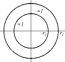
Fig. 1. Drawing of a double-ring phase DOE

1.1. Focal field when lighting DOEs by flat-top beams

g = ^r 1 / ^r 2 ⁽ < 1).

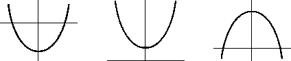
Thus, the following three configurations are possible (Fig. 2): the negative minimum (provided 0 < g <  1/ V2); the positive minimum (provided 1/ V2 < g < 1Л4/ 2 ), and the positive maximum (provided 1/ 4 2 <ц< 1). The fourth configuration, i.e. the negative maximum , is impossible.

The field amplitude in the lens focus plane is determined by the radially symmetrical Fourier transform as follows:

a)                    b)                    c)

Fig. 2. Layout view of the amplitude near optical axis: configurations I (a), II (b), III (c)

2            I k P r I

A(P) = JЛ(r)Jо I      Irdr , о         к f J

where A 0 ( r ) is the field amplitude in the input plane, J 0 ( x ) is the Bessel function of the zero order, k = 2 n / % is the wavenumber, % is the wavelength of an illuminating beam, f is the focal length of a lens, which is combined with the a double-ring phase DOE. In our case, we have the following:

The zero amplitude position is obtained by setting the right-hand side of Eq. (3) equal to zero; when x = k p r 2 / f, this gives the following equation:

2 g J 1 ( g x ) = J 1 ( x ).

A 0^{( r} ) =

1,0 <  r <  r , 1

- 1, r <  r <  r 2 .

The first nonzero root of this equation is considered. The equation is solved numerically by using Bessel function tables, and then, if necessary, the root curve x 0 ( g ) can be approached to the analytic curve. If we know x 0 , we can determine the radius of the dark ring as follows:

Substituting Eq. (2) in Eq. (1), we obtain the following expression for the amplitude:

f

A ^{( P )} = - p ²

^k P ^r 1 f

^^^^^^s

I k P r 2 r

^{2 1} к f

The zero-point amplitude is equal to the following:

A ( p = 0) = r ² - -^.

A (0) = 0 , when r 1 ² = r ₂²/2 ; provided r 1 ² >  r ₂²/2 A (0)>0 , otherwise A (0) <0 .

Since

A '( P ) = -

r ²d r , A '( p = 0) = 0 ,

we see that a critical point will be always in zero. The second derivative is equal to the following:

A 7P)

-

k ¹ f J

r ₁

r 2 ⁴

A 7p = 0) = -1 - I

•

-

wherefrom we obtain A " (0) = 0, when r* = r ₂ 4 / 2 ; provided r 14 >  r ₂ 4 / 2 A " (0) < 0 (maximum), otherwise A " (0) > 0 (minimum). For r* = r ₂ 4 /2 an extremum shall be flat. Thus, using the Taylor series expansion, we can prove that this will be the maximum .

Let us introduce the following notation:

P 0 =

^x 0 • ^f kr ₂

It is directly shown in Eq. (6) that at g = 0 and g = 1, x 0 = j 1,1 is the first root of the function J 1 ( x ). Thus solving Eq. (6), we obtain the following values.

Table 1. Zero amplitude position versus ring radius ratio

g	0	0.1	0.2	0.3	0.4	0.5	0.6
x 0	3.832	3.742	3.513	3.212	2.866	2.462	1.912
g	0.7	1T - 0 2	1T + 0 2	0.8	41 2	0.9	1
x 0	0.553	0	6.116	5.539	5.241	4.734	3.832

1.2. Focal field when lighting DOEs by Gaussian beams

In this case, the field amplitude in the input plane is as follows:

A ₀( r ) = e ^- ( ^{r 2 ,2} ° ^{2 )}

1,0 <  r <  r , ^{- 1, r} 1 <  r <  ^r 2 .

where о is a beam-width determining parameter. It is impossible to make exact calculations here; however, we can obtain rather close approximation. Breaking down the element into two rings, we get the following:

A (P) = r1       r2                                  r2      r2

₃ 2 I kr p I                2 г | kr p I

= e ^{2 0} J       r d r - e ^{2 0} J       r d r =

0 к ^f J r к ^f J

= B ₊ - B - = 2 B ₊ - ( B ₊ + B - ).

The sum in parentheses can be determined with a reasonable degree of accuracy using the tables given below,

if the pupil’s radius meets the condition r 2 >~ (2÷2.5) σ when an upper limit could be replaced by an infinite limit. The following formula is given in tables presented in paper [19] (p. 186).

∞ j e - px Jv (cx) x dx =

Before proceeding any further, it’s worthwhile to get at least one technique for finding the values α 1 and α 2 . The simplest method, though probably not the best one in terms of its accuracy, is a collocation method. We equal zero and edge values as follows:

__ 2     XXXX

-c2                    22

c^П e8p.              1-7

8 p ³² e     [ I ^{( v- 1)/2} ( 8 p J I ^{( v+ 1)/2} ( 8 p J

When ν =0, the formula is simply as follows:

∞c e-px J (cx)xdx = e 4p j 0 ( )        2 P

.

Using Eq. (10а), we obtain the following:

∞ _- r ²

B _{+ +} B _ = j e ' J о

r d r = σ ² e

( k ρσ ) ² 2 f ²

(10а)

We can calculate the value of B + with the specified degree of accuracy replacing a Gaussian function bell with a parabolic cone, when r 1 ≤ σ (a knee of the Gaussian curve). The case when this condition isn’t well fulfilled is uninteresting: an exterior ring has no meaningful effect. So, the result is limited to one circular hole to be lighted.

Suppose the condition r 1 ≤ σ has been satisfied. Then the following approximation should be made with a small accuracy over the range of r ≤ r 1 :

- ^{r 2}

e ^{2 σ 2} ≈ α ₁ - α ₂ r ².

The values of α 1 and α 2 depend on used approximation and they are given below. Using Eq. (12), we receive the following:

r ₁

I kr P | ( α -α r ²) J       r d r =

4                                / о                 V f J

fr Tk k P rl К =2 J α - k P 11 f J ( 1

. I Jr | , I k p r | +41 — I J ₂ 1      I a

I ^k P J I f J

r ₁ ² ) +

The overall amplitude is equal to the following:

A = ² fr^ J f ^{k p} r "¹ ( a-a r ² ) ⁺ k P 1 _V f _J 1     2 1

2                              ( k ρσ

. I fr | , I k p r |         ₂ 2Г

+ 4 ¹ J ¹ α -σ ² e ^{2 f}

V k P J   V f J

This shows that for large values of ρ decreasing is determined with the first summand and the rate of decay is identical to that one valid for lighting with flat-top beams. When r 1 =0 (no phase step), we get a trivial response:

_- ( k ρσ ) ²

A = -σ2e 2f2 , which is the Gaussian beam.

1 = α ₁, e - ( r 1 ² /2 σ ² )

2 = α ₁ - α ₂ r ₁

К = 1,

² 'a _; = (1 - e-(r'/²^) ) • 1.

I                                     r 12

Substituting Eq. (15) in Eq. (14), we obtain the following:

r ²

A = 2 & J 1 f k e r i 1 e" 2? k P V f J

J ₂

f 1

1 - e ^2o 2

+

_- ( k ρσ ) ²

-σ ² e ^{2 f 2}

VJ

The value of A ( ρ =0) can be calculated exactly without any approximations made. It equals to the following:

A ( ρ = 0) = σ ² - 2 σ ² e ^{2 σ 2} + σ ² e ^{2 σ 2} .

Providing however that r 2 is larger (see the line before Eq. (10)), the latter summand shall be neglected:

A ( ρ = 0) = σ ² ( 1 - 2 e ^{- ( r 12 /2 σ 2 )} ) .                       (17а)

Configurations will be determined according to Eq. (17a) being similar for derivatives. We write out accurate values, just as in Eq. (17), but they are less convenient for analysis due to their complexity.

A (0) = 0 , when r ₁ = σ 2ln2 ≈ 1.1774 σ .        (18)

At less values of r 1, we have A (0) <0, otherwise we have A (0) >0.

The first derivative A' ( ρ =0) equals to zero and the second one is as follows:

A ′′ ( ρ = 0) =

-

k f

' ^CT 4 -

V rL 1

⋅

+ 0,5 o ²( r ₂ ² + 2 o ²) e ^{2 a} 2 .

J

_- r 1² σ ²( r ₁ ² + 2 σ ²) e ^{2 σ 2} +

With disregard for the latter summand, we get the following:

ГИ2

A ( P = 0) = - V f J о •

I

° ²

V

-

zL 1

( Г 1 ² + 2 о ²) e ² ° 2 ,

(19а)

J

A ′′ (0) = 0, when r ₁ ≈ 1.832 σ , (20) where 1.832 is the root of the equation 1 = ( x ²+2) e ^{– x 2/2}. This corresponds to the flat maximum at a smaller vale of A" (0)>0 (minimum), otherwise we have A" (0)<0 (maximum). Configuration change takes place similarly as in case with flat-top beams (Fig. 2)

Configuration I:

Configuration II:

Configuration III:

r 1 < 1.1774 σ ;

1.1774 σ <  r 1 <1.832 σ ;

r 1 > 1.832 σ .

It is difficult to compare edges obtained from fully exact expressions because of the fact that there are two radii, not one, in exact expression. However, we can compare them with those ones that will be used in Eq. (16). Using two summands of the Taylor series ( J 1 ( x ) ≈ ( x /2) – ( x ³/16), J 2 ( x ) ≈ ( x ²/8) – ( x ⁴/96)), the near-axis amplitude can be conceived of as follows:

A ≈

r 1 ²

Г     - -L )

1 + e ^{2 a} 2 -a ²

V J

_- r ₁

1 + 2 e ^{2 σ 2}

A

σ ⁴ +

Though Eq. (21) is approximate, the zero value is exact; it equals to the following:

F

A (0) = - - 1 + e

-L ) 2 a ²

-

σ 2 ,

V

J

wherefrom

A (0) =0 at r 1 ≈ 1.15 σ , (22) where 1.15 is the root of the equation x ²(1+ e ^{– x 2/2}) = 2; it is somewhat less than the factor given in Eq. (18). The second derivative is equal to the following:

A ′′ (0)

_- r 1 1 ₊ 2 e - ( r 1² /2 σ ² ) ₊ σ 4

A ′′(0) =0 at r 1 ≈ 1.687 σ , (23) where 1.687 is the root of the equation x ⁴(1+2 e ^{– x 2/2}) = 12; it is less than the factor given in Eq. (20). Overall, the area of configuration II is narrower than that one obtained by exact calculation. It should be pointed out that the factor given in Eq. (22) and especially in Eq. (23) is larger than permitted; this is necessary to make the approximation mentioned in Eq. (12), on the basis of which Eq. (16) has been obtained, be good .

Zero values of Eq. (16) shall be determined using the below tables. With the use of

x= (kρr1/ f); r1 =µ⋅σ we have A (ρ) =0 be written as follows:

2µ2 ⋅ J1(x) ⋅e-µ2/2+ x                                        (24)

₊ 4 _µ 2 _⋅ J 2 ( x ) _⋅( 1 _- e -µ ² /2 _{) =} e - x ² /(2 µ ² ) .

x ²

The equation is solved for x at given µ . If we know the root of x 0 , the radius of the dark ring is determined as follows:

ρ ₀

x ₀ f ---------- . -------------

.

µ k σ

In contrast to Eq. (7), a real factor is not x 0 itself, but x 0 / µ . That’s why we added a proper line in the table of roots of equation (25) (implication of one more line will be clarified below).

wherefrom

Table 2. Zero amplitude versus circle-and-beam radius ratio

µ	0	0.1	0.2	0.3	0.4	0.5	0.6	0.7	0.8	0.9	1	1.1	1.15
x 0	0	0.3043	0.51	0.669	0.79	0.879	0.936	0.961	0.948	0.888	0.755	0.464	0
x 0 / µ	∞	3.043	2.55	2.23	1.975	1.757	1.56	1.372	1.185	0.986	0.755	0.422	0
2 µ - ln µ	0	0.3035	0.5075	0.658	0.766	0.833	0.858	0.836	0.756	0.584	0	–	–

In contrast to the flat case, when µ was within the range from 0 to 1 (though it had another definition there), here µ can theoretically possess any positive value, however really meaningful values are limited: when µ >2÷2.5, this is equivalent to near-zero values with the amplitude sign reversal. Besides, Eq. (16) and therefore Eq. (25) are obtained on the assumption that µ <~ 1. Anyway, the values larger than 1.15 (see. Eq. (22)) are not particularly of any interest.

It is apparent from the above table that with reducing µ the radius ρ 0 goes up with no limit as it must be. The amplitude constraint tends to the Gaussian curve that possesses no zeros.

With small µ we can also determine the root value without the benefit of the tables. The right-hand side of the equation (24) at µ→ 0 and with a fixed value of x tends to zero much faster than the left-hand side; therefore x should be small, too. In this case, we can make the following approximations on the left-hand side of the equation:

• -µ ² /2 -µ ² /2 ^µ J 1 ( x ) 1 J 2 ( x ) 1

e ≈ 1; 1 - e ≈ ; ≈ ; ≈ .

2 x 2 x ² 8

Then the left-hand side of the equation will be averagely equal to the following:

2 1           2 1 ^{µ 2}       2 1 4      2

µ 2 + µ 8 2 =µ +4µ ≈µ , so, we get the following equation:

µ ² = e ^{- x 2 /(2 µ 2 )} → x ₀ = 2 µ - ln µ .                  (26)

The ratio x ₀ / µ = 2 - ln µ goes up with no limit when µ→ 0.

2.    Numerical simulation results

Numerical simulation was implemented under the flat incident beam with the following parameter: the outer radius is r 2 = 100 λ ( λ is the wavelength of incident radiation equaled to 1 µm); the lens focal length is f = 400 λ . Let S denote a ratio between the side lobe intensity and the centered intensity. The results are given in Fig. 3-6.

As we can see, when the size of the central light spot decreases, the energy goes out of it into a peripheral ring.

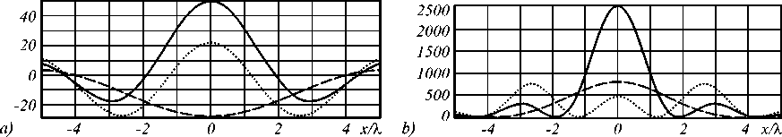
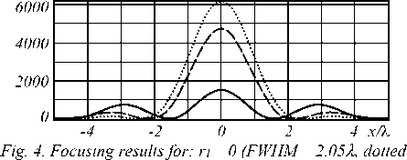
FWHM = 1.2 λ , S = 1.6). Amplitudes (а) and intensities (b) are shown

Fig. 3. Focusing results for the element with phase step radius r 1 = 0.6r 2 : the element’s interior-part field (dashed line, FWHM = 3.43 λ , S = 0.015), the element’s front-end field (solid line, FWHM = 1.74 λ , S = 0.123) and their superposition (dotted line,

line), r 1 = 0.25r 2 (FWHM = 1.91 λ , dashed line), and r 1 = 0.5r 2

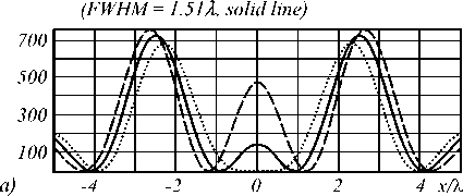
Fig. 5. Focusing results for: r 1 = 0.6r 2 (FWHM = 1.22 λ , dashed line), r 1 = 0.65r 2 (FWHM = 0.96 λ , solid line), and r 1 = 0.7r 2

Fig. 5 shows that it is also possible to obtain very small sizes for the central spot through its very low brightness and growing side lobes.

If we compare numerical simulation results with theoretical calculations, they should nearly coincide. Sources of discrepancy are as follows: computational errors in solving the Eq. (6); computation errors of numerical simulation; visual accuracy of determining the zero position in graphs obtained by simulation.

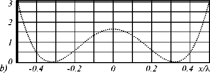
(FWHM = 0.35 λ , dotted line) (а); central part for r 1 = 0.7r 2 (b)

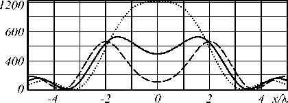
Fig. 6. Focusing results for: r 1 = 0.75r 2 (dashed line), r 1 = 0.8r 2 (solid line), r 1 = 0.85r 2 (FWHM = 3.9 λ , dotted line)

By parameter values from Eq. (7) used in simulation, we get the following:

ρ 0 = (0,637 x 0 ) ⋅λ . (27)

Values of the radius of the first dark ring calculated by Eq. (27) and determined according to certain intensity graphs obtained from simulation are shown in Table 3. Values of x 0 are taken from Table 1 or obtained by interpolation.

Table 3. Comparison of zero points discovered theoretically and by simulation

µ	0	0.25	0.5	0.6	0.65	0.7	0.75	0.8	0.85
ρ 0 as in (27)	2.44	≈2.148	1.568	1.218	≈0.785	0.352	≈3.726	3.528	≈3.289
ρ 0 as in graph	≈2.5	≈2.2	≈1.5	≈1.2	≈0.85	≈0.32	≈3.75	≈3.5	≈3.3

Values of the radius are given in units of wavelength . Designated values mean the use of linear interpolation. Note that for µ = 0.25 and 0.85 interpolation produces adequate accuracy; for µ = 0.75 – mean accuracy, and for µ = 0.65 – low accuracy. This is due to the fact that interpolation accuracy increases when a derivative of the interpolated function approximates a constant.

It may be concluded that compatibility between theoretical calculations and numerical simulation results is very high.

Conclusion

Analysis of operation of double-ring optical elements allowed us to come to the following conclusions:

• 1.    Three significant configurations for amplitude (two – for intensity) are possible near optical axis. Edge configurations are supposed to be the centered zero value

• 2.    Equations are derived for the first zero intensity position. Tables of their roots are given.

• 3.    Numerical simulation implemented for the case of incident beams has fully confirmed theoretical predictions.

and the largest flat-topped value similar to the configuration mentioned in paper [1]. A type of configuration is determined by the ratio between inner and outer radii at flat beam incidence or by the ratio between inner radius and width of the Gaussian beam.