Fuzzy SLIQ Decision Tree Based on Classification Sensitivity

Published Online August 2011 in MECS

Decision tree has been widely used in Data Mining from feature-based records for classification and decision making. Various algorithms have been developed to construct decision trees from data, such as ID3 [22], C4.5 [23], SLIQ [9] and so on. A notable characteristic of these traditional decision tree inductions is that node split is crisp. ID3 proposed by Quinlan works well on sets of examples only with nominal or discrete attributes value, while C4.5 and SLIQ are better for quantitative data. These traditional algorithms have excellent performance in extracting knowledge. However, they usually suffer from some defects. For the induction of classic crisp decision trees, training data is recursively split into a collection of mutually exclusive sets till all the examples at a node belong to the same class. Obviously, the split of test node has sharp boundary. Consequently, small changes in the attribute values of unseen data may lead to sudden and inappropriate class changes according to rules extracted from tree which is generated by these traditional algorithms. Apparently, this doesn’t conform to the way of human thinking.

With the seminal work of Zadeh, fuzzy set theory [15] has a valuable extension to traditional crisp decision trees and the fuzzy counterparts of traditional heuristics of induction of crisp trees have been proposed [12] [24]. Fuzzy decision trees induced by the fuzzified heuristics well process the data that cognitive uncertainties, such as vagueness and ambiguity, are incorporated into. The fuzzy trees greatly make improvement in their generalizing capability. For fuzzy decision trees, one of most important differences from crisp ones is that all training examples belong to one node with membership degree ranged on the interval [0, 1], but one example completely belongs to a node or not for crisp trees. Each example at current test node goes into every child node of the node with membership degree (∈[0, 1]) in respect to attribute selected at the node. In other words, there exist gradual transition regions on domain of values of selected attribute. Another notable difference between crisp decision trees and fuzzy ones is that all rules extracted from fuzzy tree are used for the final classification of each unseen example, however, only one rule for crisp decision trees.

In the process of constructing fuzzy decision tree from training examples, the determination of membership function installed at each test node is critical, that is, how the induction algorithm ascertains the membership degree of each example to child nodes is central to any induction algorithm within fuzzy environment. The construction of membership function has generally been determined with opinions of experts, this more conforms to real-life condition. However, the way is low efficiency, and experts usually can not propose appropriate membership functions to given some complex data sets [27]. The fact mentioned above brings great difficulty to the construction of fuzzy decision tree. In view of this, more attention is paid on the research of automatic construction of fuzzy membership functions and fuzzy trees. In this paper, we will also give much concern to automatic construction of membership functions characterized with some parameters. For existing algorithms of fuzzy trees induction, final split of node depends on fuzzification of candidate attribute. When candidate attribute is numerical, it needs to be fuzzified into linguistic terms. Each child node of current node corresponds one of linguistic terms of selected attribute. This paper restricts the scope of our discussion to datasets that only consists of numerical attributes.

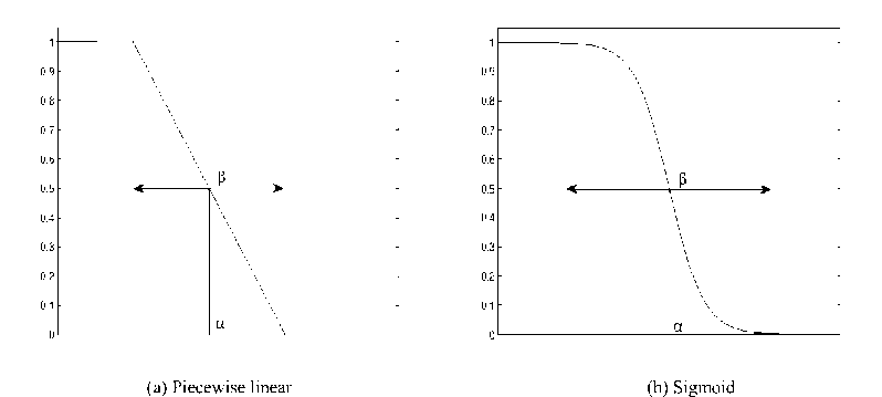
Figure 1. Examples of discriminator function.

Moreover, the number of linguistic terms of each attribute is limited to 2. Therefore, this paper focuses on fuzzy binary trees. According to topology of binary trees, we usually call membership function installed at test node discriminator [2] or dichotomy [3], its value is ranged from 0 to 1. The task of automatically determining discriminator is specifying two parameters: α , the location of split point that is the split threshold at a test node of a decision tree, and β , the width which measures the transition region on the attribute selected at that node, as shown in Fig. 1. Existing approaches of automatically determining discriminator in fuzzy decision tree is mainly divided into three categories:

♦ Optimization technologies, such as local optimization and global optimization, are utilized to construct membership function. The way usually needs a lot of calculations. Further more, the results of these optimization technologies are sensitive to sets of examples. More details are found in [2], [3], [5].

♦ Some methods based on characteristics of data is popular. The characteristics generally include probability distribution [13] and statistical characteristics [1] of data. Obviously, these methods are superior to the methods based on optimization technologies in computation. Their implementation are also simpler. In this paper, sensitivity based discriminator function, which this paper proposes, just depends on statistical characteristics of data.

♦ Constructing fuzzy discriminator function with intelligent method. For example, Kohonen’s feature-maps algorithm is used to determine membership function [4][14].

The paper is organized as follows: Section 2 describes motivation to the proposed methods. Section 3 introduces proposed method to construct dichotomy functions. Section 4 applies proposed technique to several datasets from UCI machine learning repository and presents a comparison between the two algorithms respectively proposed by us and B. Chandra [1] and mentions related work. Section 5 provides some discussion on the proposed method.

• II.    Motivation

Above all, let us review some basic concepts and related representations. Let U denote the universe of all examples in a real-life dataset. For a fuzzy subset A (e U), we use ^ to refer to its membership function, and denote by ^^ (e) membership degree of a example e in fuzzy set A. Note that ^U (e) = 1 by definition. The cardinality of a fuzzy set is defined as the sum of membership values of each element in Ã, and denoted by

||A || = 2 a ^ a ( e ) [15]. For each example e in dataset,

the value of its the i th predictor attribute is denoted by a i ( e ), the domain of values of attribute a i is defined as the set including all values of this attribute, we denote it by dom ( a_i ). The set of classes of examples is denoted by C , and each class denoted by c i ( e Q.

Traditional heuristics attempt to select the attribute that can most greatly reduce the impurity of examples belonging to current test node. In the construction of fuzzy decision tree, the candidate attributes, their discriminator functions having steeper transition regions, are more easily selected as split attributes at test nodes [2] [3] [5][28][29]. Since the attributes that have sharp discriminator can more crisply split examples in current test node into two child nodes, and the proportion of I^ = 2eeC,MLS (e) to P|| = 2eeLS ^LS (e) usually becomes larger (where fuzzy set LS consists of examples belonging to the left child node, Ci consists of examples in LS which belong to same class ci, consequently, ||A = 2e6C A L S (e) is the cardinality of C, and

I ^A | = 2 e . LS

^LS (e) the cardinality of LS), that is, the set of examples in the left child node is purer. That is similar to the right child node. Hence, the attributes that have steeper discriminators can more reduce the impurity of

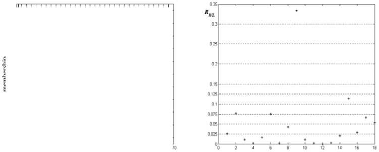
(b) R WL of attribute a i .

Figure 2.

(a) Discriminator of attribute a i

examples, this is why the kind of candidate attributes are more inclined to be selected as split attribute. The pathological character of heuristics used in the construction of fuzzy trees is external manifestation of the convexity property of heuristics [2] [3][28][29], and it has been verified empirically and theoretically. Therefore, some modification to traditional heuristics are proposed to avoid the pathological character in induction of fuzzy decision trees.

SLIQ, Gini Index based algorithm, is popularly used to construct crisp trees. It uses pre-sorting technique and breadth-first tree growing strategy in induction of crisp decision trees. SLIQ can obtain higher accuracies by classifying larger training datasets which can not be handled by other classifiers. B. Chandra has integrated fuzzy set theory into SLIQ by fuzzifying Gini Index [1] [18]. The performance of G-FDT algorithm proposed in [1] outperforms its crisp counterpart with respect to classification accuracy and the size of decision tree.

Let’s describe some of the details of G-FDT algorithm. What is most worth noting is the automatic construction of discriminator functions installed at test nodes. In induction of fuzzy binary trees, two kinds of discriminator are favored: Piecewise linear discriminator and Sigmoid discriminator shown in Fig. 1, and G-FDT algorithm uses the Sigmoid discriminator functions which could behave better in term of convergence properties than piecewise linear discriminators [3]. The construction of discriminators of G-FDT is to determine the width parameter, α , and split point, β , as described above. Now, let’s show the expression of discriminator used by G-FDT:

1 + e - ° ( а ⁽ e ^)- “ )

where σ is the standard deviation of values of attribute ai of all training examples. Equation (1) is the discriminator of candidate attribute ai at current test node N. Examples in N is fuzzified into two fuzzy sets or linguistic items with candidate attribute ai, and membership functions of the two fuzzy sets is v and 1-v, respectively. If ai is selected as split attribute of N, each example e in N(The degree of membership of e to N is denoted by д (e), where N% is a fuzzy set corresponding to N) goes into left child node of N with membership д# (e) v (a (e)), and the right with ^N (e)(1 - v (a (e))). Fig. 1 (b) shows the curve of 1 - v.

The parameter β , width of transition region of discriminator defined in domain of attribute values, dose not appear in (1). Actually, there exists a function mapping between β and σ . With the value of σ increasing, the width of transition region of the discriminator is smaller and the shape of discriminator is steeper. On the contrary, the opposite is true. In other words, the width β is a decreasing function of σ . The function is denoted by f , that is, the expression of the function is

β = f ( σ ) (2) Therefore the determination of the width β depends on the determination of σ , or the steepness of the discriminator function depends on σ . Hence, the task of constructing discriminators used by G-FDT is specifying parameter α and σ . Apparently, σ is directly determined by computation. G-FDT evaluates every pre-selected split point value with fuzzifying Gini Index to determine the best split point α *.

Although the way of determining discriminator at each test node is fairly simple, it suffers some defects. We are now analyzing the shortcomings of the method: For most datasets (as mentioned above, we restrict our discussion to the datasets of which examples only have numeric attribute value. It is also the case for G-FDT), the standard deviation of attribute values of training examples is greatly large especially for the datasets that have attributes values of which the interval has relatively great length. In order to describe the degree of steepness of discriminator, we use the ratio of the width of transition region of a attribute ( a i ) discriminator to the length of interval of this attribute, where the interval is [min{ a_i }, max{ a_i }], and min{ a_i } is the minimum of dom ( a_i ), max{ a_i } is the maximum of dom ( a_i ). Hence, the length of interval of this attribute a i is max{ a i } - min{ a i }.

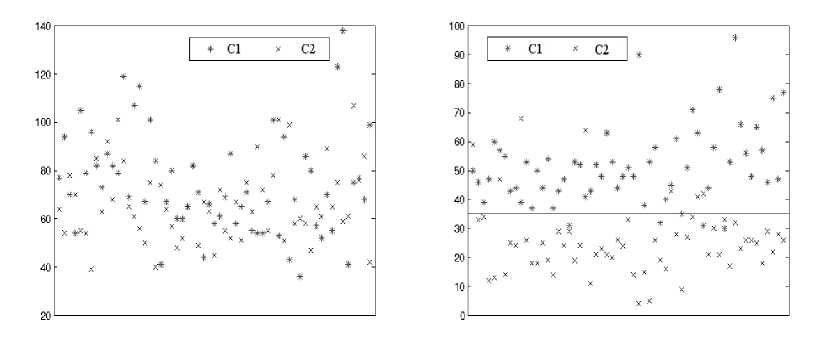
(a)

(b)

Figure 3. Distribution of attribute values.

The width of transition region of discriminator function v is defined by

β = | a i ( e 1 ) - a i ( e 2 ) | , where v ( a i ( e 1 )) = 0.99; v ( a i ( e 2 )) = 0.01. Thus, the ratio(denoted by R WL ) can be defined as

R...=в

We now present steepness of attribute discriminators determined by G-FDT with vehicle silhouette dataset which is taken from UCI machine learning repository. According to Fig. 2 (b), we can conclude that almost discriminators constructed by G-FDT are very steep, that is, the width of transition regions of almost discriminators is very small. We take R WL =0.075 for example, the paper gives the discriminator in Fig.2 (a). The partition of training examples approximates to crisp partition. These discriminators approximate to crisp discriminator used in traditional crisp decision trees. Actually, the fuzzy decision tree induced by G-FDT collapses into a crisp decision tree. This does not meet the original intention of inducing fuzzy decision trees.

In practice, not every candidate attribute corresponds to a very steep discriminator constructed by G-FDT. The degree of steepness of some discriminators generated by G-FDT is acceptable to human thinking. Fuzzy trees assembled from these discriminators present excellent performance in terms of classification accuracy and size. However, as mentioned earlier, the candidate attributes, possessing discriminators of which transition regions are not very steep, are seldom selected as split attribute according to G-FDT. This apparently enlarges the possibilities that the fuzzy decision tree induced by G-FDT collapses into a crisp decision tree.

Generally speaking, the test nodes the fuzzy trees generated by G-FDT usually have such discriminators that have too narrow transition regions. Thus, the trees induced by G-FDT hardly present fuzzy decision tree’s advantage that fuzzy trees are good at handle the data with cognitive uncertainties and noises. In view of this, we manage to propose a method of generating discriminators to make up for the drawback. This method should meet the following tow requirements:

Firstly, the proposed method makes sure that steepness of discriminator is not very large and is acceptable. This directly reduces the possibility that the fuzzy decision tree collapses into a crisp decision tree.

Second, the method can make sure that the attributes with higher classification capability have relatively steeper discriminators. Thus, the kind of attributes are easy to be selected as split attributes according to fuzzifying classical heuristics. This can also try to overcome the pathological behavior of the attribute tests at split nodes inclining to select a crisp partition.

It is a critical problem how we measure classification capability of each candidate attribute. It is also central issue of next section.

Ш. Sensitivity Degree Based Induction Algorithm

In this section, we will introduce our proposed method that is used to automatically build discriminator function for each candidate attribute.

We now firstly give an example of distribution of attribute values, taking a dataset as example. Examples of the dataset here can be categorized into 2 classes (denoted by Class 1 and Class 2, respectively). Fig. 3 (a) and (b) present value distributions of two attributes of examples in the dataset with class, respectively. The vertical coordinates in each coordinate system correspond to the values of corresponding attribute, and Class1 is denoted by * point, Class2 by × point.

One intuitively thinks that the attribute shown in (b) can better categorize examples than the attribute shown in (a), because the points above horizontal line in (b) mostly belong to examples which belong to Class1, the ones below the line mostly belong to Class2. We here think that the attribute shown in (b) is more sensitive to final classification results of unseen data. The more sensitive candidate attributes should be understandably selected as split attributes in construction of fuzzy trees. Now, what we concern is that how the sensitivity of each of attributes is measured. As can be seen from Fig. 3 (b), the difference of the two mean values of attribute values of examples (respectively belonging to Class1 and Class2) is obvious. Hence, we can specify the sensitivity degree of attributes to classes of examples according to the difference mentioned above.

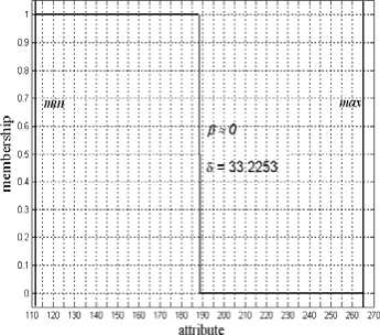
Fig. 4 presents a distribution of another attribute of examples belong to the same dataset. Apparently, the attribute can also categorize examples well, and the attribute is fairly sensitive to categories of examples. However, it is difficult to determine the sensitivity degree with the difference mentioned above, because the difference between mean values is slight Another index needs to be raised in order to overcome drawbacks brought by only using mean values of attribute values The standard deviation measures the spread of the data about the mean value. It is useful in comparing sets of data which may have the same mean but a different range. Therefore standard deviation certainly can measure the sensitivity degree of attributes especially for the case in Fig. 4.

We temporarily center our attention on datasets that have two categories. Then, datasets of examples having more than two categories are discussed later. Consequently, the sensitivity degree (denoted by λ ) of each attribute a_i to classes in C (where || C || = 2) is a function, φ , with respect to mean value μ_i j and standard deviation σ ij of the attribute of examples belonging to same class c j ∈ C (where j = 1, 2). Thus, the sensitivity degree λ ( a_i ) of attribute ai to classes is denoted by

2 ( а^ = ф ( u 1 1 , 4 1 , u i ₂ , a _i2 ) , (4) Where

^A j = C l l^ e ) ⁽⁵⁾ and

⁴j = I E[ a i ⁽ e ^)- ^ j ]² /(II C II^- 1 ), ⁽⁶⁾ V ^{e €} C j

C j (a crisp set) consists of examples which belong to class c j ( j = 1, 2), and || C j || is the number of elements in C j . In order to determine the sensitivity degree ( λ ) of a i with differences of mean values and standard deviation values, we firstly define a function δ ( x 1 , x 2 ) to measure the differences between x 1 and x 2 , where x 1 , x 2 are arbitrary real numbers:

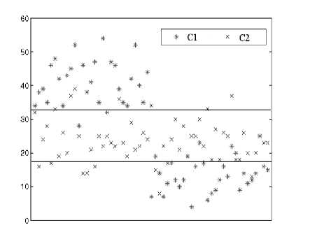
Figure 4. Distribution of attribute values. Copyright © 2011 MECS

max { x , , x 2 }

Case1: £ (xP x2) = —4-----г, x. x2 > 0, min { x1, x 2}

Case1: when x 1 x 2 ≤0,

• 1 .0, | x 1 - x ₂1 <  0.25 x boundary

• 1 .5, | x 1 - x ₂1 >  0.25 x boundary

  £ ( x . , x 2 ) = '

  
  

Based on the fact that σ ij plays more important role in determining φ when the difference of μ ij is small. We propose specific mathematical expression of function ' for datasets having two categories:

2 1                                   2

• ² ( a i ) = d 1 4 ( A i , A 2 )^- 1 ] + 77-------7 4 ( ^ 1 , ^ '2 ) - ^{1 ]}

• 4 (A1, A2)(7)

Evidently, λ ( a i ) ≥ 0 is true. When μ i 1 = μ i 2 and σ i 1 = σ i 2 , λ ( a i ) = 0. In other words, when the attribute ai has relatively approximate or same values of mean and standard deviation of attribute values with respect to the two categories of examples, ai are not sensitive to categories of examples as a whole, and examples at current test node is not well categorized with attribute ai. Moreover, the parameter ξ is used to adjust the values of λ ( a i ), trying to avoid the fact that the values of λ are extremely large or small. In here, we make ξ = 5 on the basis of the experimental experience.

According to (7), we can draw such a conclusion that the more approximate the values of mean of attribute values with categories of examples are, the less the values of mean of attribute values contribute to value of λ ( a i ), the more important the values of standard deviation of attribute values with categories of examples play role in measuring the sensitivity degree of ai to categories of examples, and vice versa. Therefore the proposed method, which is used to measure sensitivity degree of attributes to categories of examples, certainly works well for circumstances encountered in Fig. 3 and Fig. 4.

For the sake of understanding, previous parts of the section mainly present our proposed method under this circumstance that examples are only categorized into two categories. We now give details about measuring sensitivity degree of a attribute to categories of examples in datasets of which examples can be categorized into more than two groups. Above all, suppose that the currently considered datasets have N ( N > 2) classes of examples. Under the enlightenment of the way of determining sensitivity degree for datasets having two classes of examples, we consider that the distribution of attribute values with respect to any two of categories of examples can contribute to the sensitivity degree of the attribute ai to categories of examples. Consequently, we define the sensitivity of ai with respect to any two categories c_m , c_n ( ∈ C ), and it is denote by λ ( a_i , c_m , c_n ):

• ² ( a i , c m , c n )

₂ (8) ---7 44 m , ^ ,n ) - ^1]2 A n )

= Л 4 ( A m , A n ) - 1 ]

12 ___________ 1

^{+ 4} ( A m

Where μ ij and σ ij ( j = m , n , and m , n ∈ {1, 2, …, N }) are same as (5) and (6), respectively. Finally, we obtain λ ( a i ), the sensitivity degree of ai to all categories of examples,

TABLE I.

C lassification A ccuracy

No.	Dataset	NA	NC	G-FDT Average accuracy ± std. dev.	SG-FDT Average accuracy ± std. dev.
1	Haberman	3	2	72.58±7.79	74.15±8.95
2	Blood transfusion service	4	2	77.95±3.88	79.95±4.88
3	Balance scale	4	3	84.03±8.28	89.29±3.57
4	Australian credit approval	14	2	78.41±4.76	81.59±2.56
5	Vehicle silhouettes	18	4	70.12±4.58	72.47±5.40
6	Contraceptive Method Choice	9	3	52.00±5.34	52.48±3.39
7	Pima Indians diabetes	8	2	74.94±5.97	74.09±4.87
8	Wine	13	3	88.89±4.45	89.38±9.61
9	Statlog(Heart)	13	2	75.33±6.71	77.78±6.05
10	Dermatology	34	6	75.42±8.33	94.83±5.18
11	Parkinsons	22	2	82.95±13.40	84.00±10.69
12	Liver	6	2	60.48±14.76	69.28±6.50
13	Image segmentation	18	7	89.29±5.41	90.71±6.19

NA: number of attributes; NC: number of categories.

by computing the arithmetic mean of values of λ ( a i , c m , c n ) for any two ( c m , c n ) of categories of examples:

M^ai ) ⁼ —Г7 X M a , Ci,C t) (9) ⁽ *) C ( N ,2 ) _Cm ^ . c ⁽ j k’

Where C ( N , 2) is the number of all combinations of any two categories c_m , c_n in C (the set of categories of examples, and || C || = N ).

Undoubtedly, the (9) will evolve into (7), when N = 2. Hence, (9) can be used to measure the sensitivity degree of attributes to categories of examples that are classified into two or more classes ( N ≥2). In addition, boundary is the mean of μ ij ( j = 1, 2… N ) when we compute the differences of mean values, and the mean of σ_i j ( j = 1, 2, …, N ) when we compute the differences of standard deviation values.

As mentioned above, the more sensitive to categories of examples attribute is, the better examples are split with the attribute, that is, the higher classification capability the attribute has. Therefore candidate attributes with larger sensitivity degree are more inclined to be selected as test attributes at test nodes, these attributes should correspond to discriminator functions with steeper transition regions. Thus, we now define proposed discriminator function as bellow:

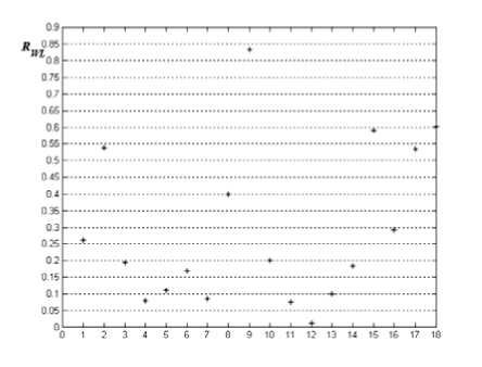
Figure 5. Degree of steepness of discriminators constructed by proposed method..

where λ ( a i ) and α are same as above. The parameter ρ plays similar role as parameter ξ in (8). Generally, ρ = 1.35 according to experiments, so ρ is used to enlarge the value of λ ( a i ). In meanwhile, (2) evolves into:

β = f ( ρλ ( a i )). (11) In other words, the width β of transition region of discriminator indirectly depends on sensitivity degree of corresponding attribute.

As stated above, the proposed discriminator well conforms to the second requirement mentioned at the end of Section 3. We also present the values of R WL (Fig. 5) of attributes of examples in same dataset in order to make sure whether proposed discriminator conforms to the first requirement or not. From the analysis of Fig. 5, the transition regions of most discriminators generated by our proposed method slope gently, this greatly reduces the possibility that induced fuzzy trees collapse into crisp decision trees. There also exists some of attributes that have steeper discriminators, but these attributes are sensitive to categories of examples, therefore steeper discriminators make corresponding candidate attributes prone to be selected as split attributes. It is obvious that our proposed method, which is used to generate discriminators, well satisfy the requirements referred to in Section 2.

Finally, we modify the G-FDT by substituting our proposed method of constructing discriminators for the one of G-FDT proposed by B. Chandra, and the fuzzy inference mechanism of our proposed algorithm is the same as the one used in [1], so called “× - × - + method” [12]. Thus, the version of modified G-FDT is our proposed fuzzy decision tree algorithm called sensitivity degree based fuzzy SLIQ decision tree algorithm (called SG-FDT for short).

• IV.    Empirical Results

In order to reveal the performance of our proposed fuzzy trees algorithm, we present comparison between G-FDT and SG-FDT in terms of classification accuracy, size of induced fuzzy decision tree and time taken to construct decision tree, using 13 datasets from the UCI

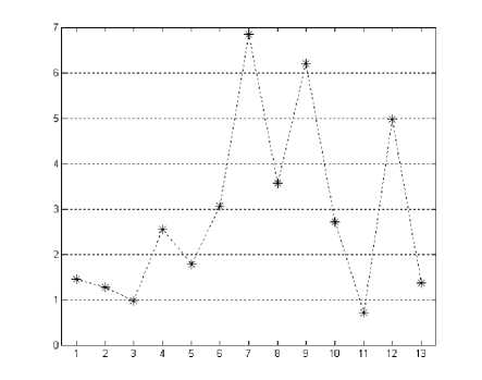
Figure 4. Distribution of attribute values.

machine learning repository. We acquire all empirical results according to 10-fold cross validation.

The comparison in classification accuracy is presented in Table I. Apparently, almost all accuracy results for SG-FDT are better than those for G-FDT, and the increase of accuracy on Dermatology dataset, Liver and Balance scale dataset is very obvious.

The comparison in sizes of induced trees is presented in Figure 6. Vertical ordinate of each point in Fig. 6 is the ratio of size of tree for SG-FDT to that for G-FDT. As shown in Fig. 6, the nodes of trees induced by SG-FDT are usually much more than ones of trees induced by G-FDT, it is hardly accepted. As mentioned in Section 2, the fuzzy decision tree induced by G-FDT usually collapses into a crisp decision tree, but the fuzzy trees induced by SG-FDT do not do that. Actually, the fact, which is referred to in many related literatures, is that the size of fuzzy tree induced with fuzzifying heuristics will be much more than that of crisp tree induced with corresponding traditional heuristics if the construction of decision trees does not include the usage of pruning technology. Therefore we can explain why the sizes of trees induced by SG-FDT are usually much larger than ones of trees induced by G-FDT. Similarly, the time taken to construct tree with SG-FDT is more than that with G-FDT.

• V.    Conclusion

One method of specifying discriminator is proposed according to the pathological character of traditional heuristics in this paper. With the method, our sensitivity degree based fuzzy SLIQ decision tree algorithm (SG-FDT) well overcomes drawbacks of G-FDT, and it can induce real fuzzy trees. That is what G-FDT seldom can do. In addition, our proposed algorithm outperform G-FDT algorithm in term of classification accuracy.