GAFBone: A New Backbone Construction for Increasing Lifetime in Wireless Sensor Networks

The wireless sensor networks (WSNs) generally consist of hundreds or thousands of sensor nodes which have limited processing ability, embedded memory and the small power unit. These nodes are being deployed randomly in the area for detecting and monitoring tasks. The mentioned networks have various applications: military and civil, targeting, nuclear biological, agriculture, disaster management like floods, volcano, and battlefield surveillance, to name but a few [1]. Because of the extensive range of applications, these networks are attractive research areas which have received more attention in recent years.

The main function of these tiny sensors is gathering data from the environment, and sending them either to each other or directly to an external base station (BS). For data collection, a typical node equipped with appropriate sensors which sense physical phenomenon such as light, acceleration, pressure, temperature, humidity, etc. This layer can be adjusted to the application by use of the versatile processing the node has [2].

When a node senses the demanded data from surrounding, reports it to a remote base station for final processing. Since the nodes are distributed in a large region, the distance between nodes and base station may be greater than the maximum transmission frequency. As a consequence, other nodes participate in propagation of the sent packets, and the data to be routed through several intermediate nodes to reach the destination. In other words, routing the packets in wireless sensor networks is very important issue which has significant impact on the efficiency of such networks. There are many routing protocols are presented in some literatures that can be categorized into three main groups: data centric, hierarchical, location based protocols [3]. Data centric protocols are based on the queries which sent by the sink to the certain regions. The sensors located in the selected area propagate the requested information when sense the special events. In this kind of protocols, there are some attributes to specify the properties of data. Flooding [4], SPIN [5], Directed Diffusion [6], Gradient-based routing [7] are some examples of this group. High rate traffic in single-tier network can lead to overloading in gateway. This problem causes other potential difficulties like latency in communication, information redundancy in the nodes and consumption energy. Hierarchical routings are introduced to decrease these obstacles. The main aim of the second group is formation the nodes into several clusters according to remained energy and nodes’ location. Each cluster has a node known as a cluster head which typically has the most energy reservation and selected by the routing algorithm. The members of each cluster communicate with each other in single-hop, and can reach to cluster head directly. Take, for example, LEACH [8], PEGASIS [9], and TEEN [10]. In fact, the principal concern of these algorithms is selecting the proper node for cluster head which causes to enhancing the network life time. Finally, the third group of routing protocols considers the location of nodes for routing the packets. These methods designed under an assumption that each node equipped with a location acquisition devise such as GPS. The idea is declining propagation of control packets due to using location information in forwarding data packets. One the famous protocol in this category is GAF [11] that is energy-aware, and in this paper we’ve improved it by constructing backbone. There are also other schemes such as MECN [12] and GEAR [13] in this order. These protocols not only designed for mobile ad hoc networks but also well applicable for wireless sensor networks where there is less or no mobility.

Besides the routing protocols, maximizing the network lifetime is one of the core challenges in wireless sensor researches. Since sensor nodes have restriction in power supply, and mostly it is impossible or impractical to replace the exhausted battery, the researchers make an effort to design energy efficiency algorithms. Constructing backbone is a mechanism to extend the network lifetime. In this study, we focus on the design of backbone structure for GAF routing protocol to make it more energy-efficient.

The reminder of this paper is organized as follows: Section II briefly discusses nodes’ energy consumption statistically, and classifies backbone-based algorithms. GAF routing protocol describes in section III. Section IV gives the details of the novel backbone for GAF. Section V provides the simulation results, and proposed the routing algorithm. Finally section VI concludes the paper, and gives direction for future works.

II.    Energy consumption issue and backbone

CLASSIFICATION

As discussed before, typical nodes have transceiver devices which let them send and receive packets. Thereby, the major source of energy consumption was from data dissemination in wireless networks. However, studies show that sensor nodes consume power not only for data communication but also when listening or idle, because the radio must be turned on for detection of incoming packets.

The literatures which study about power consumption for various types of sensors show that transmitting data spends 10~100% more energy than receiving messages. Moreover, a node in sleep state (the radio electronics powered off) uses its power 7~20 times less than one in idle state [14]. In fact, it is clear that energy consumption in idle state cannot be ignored. Consequently, if redundant nodes, which do not take part in routing frequently, transited to sleep mode the number of survived nodes would be risen. One method to reduce the number of redundant nodes is backbone-based algorithms.

A backbone is a subset of nodes which chosen for data communication, and are accessible for sleep nodes directly. The mentioned nodes that called coordinators can schedule their activation time to save the energy consumption, and maintain the connectivity of the network.

Backbone construction methods are based on minimum connected dominating set (MCDS) graph theory is known as classic NP-complete problem [15]. On the other hand, there are several backbone-based algorithms proposed in letters which some of them have been mentioned below.

The distributed clustering algorithm [16] creates some clusters in which the cluster head is in active state, and manages its own cluster’s members. The criteria of cluster head determination are different such as node id, energy residue and node degree (the number of nodes neighbors).

Grid partitioning schemes perform a procedure to divide the network zone into equal squares, and similar to clustering algorithms select a leader node in each grid for propagation of data packets. These methods are simple and have no chain effect.

MAC (medium access control) approaches are another way for making backbone structure. In MAC layer the nodes can follow periodic sleep/listen cycles [17].

Sensors can be aware of neighbor’s scheduling by exchanging synchronization (SYNC) messages. In [17] explains MAC protocols in details.

III.    Geographical adaptive fidelity (GAF)

GAF [11] is a routing algorithm which reduces energy consumption in ad hoc wireless networks. This algorithm uses location information (like GPS or other location systems [1, 6, 11]) to associate each node with virtual grid. The virtual grid is a square with width r.

After dividing the whole area into small virtual grids, the nodes distributed into the cells in such that all nodes in two adjacent grids can communicate with each other. Fig. 1 shows an example of virtual grids in GAF. All nodes in G1 and G3 can transmit packets with the nodes in G2. The idea in GAF algorithm is based on the concept of equivalent nodes. All nodes in each grid are known as equivalent nodes for routing. This method determines the equivalent nodes in each grid, and turning off unnecessary nodes while still maintaining connectivity. This determination is independent of ad hoc routing protocols and moderated by application and system information.

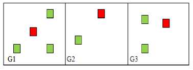
Fig 1: Equivalent nodes. (Off nodes (Green), On nodes (Red))

In GAF, nodes can transit between three states: sleeping, discovery and active which are illustrated in the state transition diagram (Fig. 2). At first, all nodes are in the discovery state. In this state the node finds neighbors in its grid by propagating discovery messages. This message contains node id, grid id, estimated node active time and node state. By use of grid size and the node location, each node can determine its grid id.

For reducing the probability of discovery messages collision, each node sets a timer for Td seconds. The discovery message transmitted after this timer expired. In that time, the node can enter to the active state. The amount of time in which the node can remain in active state is Ta. After this timeout, the node returns to discovery state to accomplish load balancing.

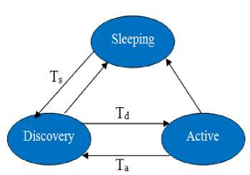
Fig 2: State transition in GAF

When a node finds out other equivalent neighbors which participate in the routing, then, it can transmit itself to the sleeping state. In this case, the node powers down its radio, but the GPS would not be turned off to avoid modeling satellite acquisition time. Sleeping duration of the node depends on the application, after this time (Ts) the node will return back to the discovery state.

GAF algorithm guarantees that there would be one active node in each grid at any time which handles the routing messages. The evaluations of this scheme show the longer lifetime in wireless sensor networks.

IV.    Roposed algorithm

• A.    GAFBone Design

In this section, a novel algorithm for constructing backbone in GAF routing, which leads to decreasing energy consumption, has been described. The proposed algorithm gets started after dividing the whole area into square cells in GAF routing. Also, assumes that the number of rows and columns that created in GAF is multiples of three which results to having better performance. The GAFBone has three phases which mentioned below.

Phase one : In GAF the sensor network divided into logical grids, and in each grid there is only one active node. Each node identified by a pair (i,j), where i and j considered as the rows and columns, respectively [18].

The grids (i, j) which have even j in their coordinates begin the step one. These grids have two neighbors in both sides left G (i, j-1) and right G(i, j+1) (Fig. 3). The initiator grid sends a query to learn the residue energy of its neighbors. Then compares them with its energy, and selects the largest amount of energy as backbone candidates horizontally. If one of its neighbors has a best condition for constructing backbone in terms of residue energy, the initiator considers it as primary backbone candidate (PBC), and notifies it by sending PBC message. Otherwise, chooses itself to continue the procedure.

Since the right neighbor of G(i,j) is the left neighbor of G(i,j+2), the intersection grid which is G(i,j+1), participates twice in this phase. If it selected as PBC for G(i,j), but does not have maximum power between g(i,j+2) vicinities, consequently, its candidacy would be discarded.

(ij-l)

1 (ij);

(U+1)

1 '(L j+2) 1

(iJ+3)

Fig 3: The intersection cell between two initiator grids

Phase two: After completing the first step, several grids have received PBC messages, and they are partial part of backbone structure potentially. The grids that their columns are multiple of three begin the next step. These central grids consider their 3*3 neighborhood, and check both vertical right (red cells) and left (green cells) vicinities. This measurement is done to make assurance that each central grid has at least one PBC in both sides left and right. If G (i, j) can find candidate cells in both sides, it quits this step, and starts the last phase of backbone instruction. Otherwise, it repeats the previous step. Unlike the first process, the algorithm selects the maximum remaining power node vertically among {(i+1, j-1), (i,j-1), (i-1, j-1)} and {(i+1, j+1), (i,j+1), (i-1, j+1)} in left and right side, respectively.

i+1, j+1	i+1, j	i+1 , j-1
i, j+1	i,j	i,j-1
i-1, j+1	i-1, j	i-1, j-1

Fig 4: Left and Right vicinity for G(i, j)

Phase three: When two steps are accomplished, some of the total grids, which have the most amount of residue energy amongst their neighbors, know themselves as the backbone structure. To ensure that the GAFBone does not have any separation and can make the appropriate routing packets in the whole network, the third procedure will be started. The initiator grids which had started the former phase fulfill the proposed algorithm.

The aim of this step is improvement the connectivity between backbone grids and non-backbone ones. To reach this goal, the central cells in 3*3 neighborhoods try to detect any disconnection between their right and left vertical vicinity. Thus, they check all backbone candidates whether they can reach each other according to their radio frequency range or not. If this communication is possible, it means that the packets can transfer through backbone structure without any loss. In contrast, if there is discreteness in these 3*3 grids, the messages which arrive, either from right or left of the central cell, they would be hindered, and there is no chance to route to the destination.

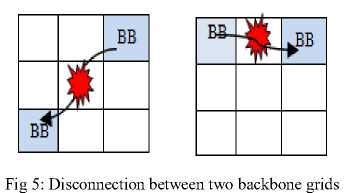
There are 10 cases in which the 3*3 grids may have disconnection. The central node analyses these states, and tries to solve the mentioned problem by turning the suitable grids on. Firstly, the central node checks its status. If it has been chosen as a backbone grid in the first phase, the columns in both sides are connected together definitely. The other nine states will be examined if the above condition does not occur. We’ve discussed only one case in details, and summarized all of ten cases in Table I.

Suppose these two conditions are met simultaneously:

{i _BB ( _R ) – i _BB ( _L ) = 0 && i _BB > i _Central}

It means the difference of the columns number of right and left neighbors becomes zero, and their columns numbers are greater than that of central. Fig. 6 shows this situation.

i+1, j+1	i+1, j	i+1 , j-1
i, j+1	i,j	i,j-1
i-1, j+1	i-1, j	i-1, j-1

Fig 6: Example of the second case

These two cells cannot communicate with each other unless with collaborating adjacent grids. There are two options in order to solve this problem. One of them is turning G (i,j) on, and the other one is activation G (i+1, j). Obviously, amongst these two alternatives the highest battery power will be selected which leads to extending the lifetime of the network.

Actually, there are other choices to join these two far backbone nodes, for example by waking the pair of {(i,j) , (i,j+1)} or {(i,j) ,(i,j-1)} up. However, it is clear that when the path will be established with less active grids, it’s not necessary to turn on redundant nodes.

Table I summarizes all ten cases, and determines the optimum number of required grids to avoid partitioning in the network.

• B.    Routing method for the proposed Backbone

After completed the backbone construction, the data transmission begins. To find a route to the destination, we proposed a routing algorithm based on α parameter which is equal to Energy/Distance.

Table 1 Checking separation avoidance

State		State
1	If G (i,j) is BB NOP	6	If {i BB(R) – i BB (L) =2 && i BB (R) > i BB(L)} MAXEnergy { G(i,j) , [G(i,j+1) , G(i-1,j)] ,[G(i+1,j) ,G (i, j-1)] }
2	If {i BB(R) – i BB (L) =0 && i BB > i central} MAXEnergy {G(i,j) ,G (i+1, j) }	7	If {i BB(R) – i BB (L) =1 && i BB (R) > i BB(L) && i BB (R) > i central} MAXEnergy { G(i,j) , G (i+1 ,j) ,[G(i-1,j) , G(i, j+1)] }
3	If { i BB(R) – i BB (L) =0 && i BB== i central} MAXEnergy {G (i,j) , G (i+1, j) , G(i-1, j) }	8	If { i BB(R) – i BB (L) =1 && i BB (R) > i BB(L) && i BB (R) == i central} MAXEnergy { G(i,j) , G (i-1 ,j) , [G(i+1,j) , G(i, j-1)] }
4	If {i BB(R) – i BB (L) =0 && i BB< i central} MAXEnergy {G (i,j) , sensor(i-1, j) }	9	If {i BB(R) – i BB (L) =1 && i BB (R) < i BB(L) && i BB (R) < i central} MAXEnergy { G(i,j) ,G (i-1 ,j) , [G(i+1,j) , G(i, j+1)] }
5	If { i BB(R) – i BB (L) =2 && i BB (R) < i BB(L)} MAXEnergy { G(i,j) , [G(i,j-1) ,G (i-1,j)] , [G(i+1,j) ,G (i, j+1)] }	10	If {i BB(R) – i BB (L) =1 && i BB (R) < i BB(L) && i BB (R) == i central} MAXEnergy { G(i,j), G (i+1 ,j), [G(i-1,j) ,G (i, j-1)] }

At the end of the last phase, each grid has a backbone table in which all active grids involved in the backbone have been determined. When a source node starts sending a query message, all active nodes in its vicinity can hear it, get this packet, and calculate the α parameter from the following equation. The Energy i and (x i , y i ) are the energy of backbone node and its coordinates, respectively. (x d , y d ) is the coordinates of the destination cell.

______ Energy_t

^(xi - x) ⁾² + (y i-ya )²

Each grid calculates this parameter, then piggybacks it with the query message, and forwards to its backbone neighbors. Each receiver node repeats this process for computing the amount of α, and next adds this value with the previous α which was piggybacked in the packets. After updating the routing parameter, the message is propagated to the next hop. This procedure continues until the query and the summation of α parameter reach to the destination grid. As there are several backbone cells can hear the transmission packet, they create the own path to the target grid. Hence, multipath from the source to the destination node will be constructed, and the final receiver node can select the optimized backward link according to the largest α value. This criterion provides assurance that demanded data would be sent back through the route with the highest energy and the lowest distance.

The below figure illustrates an example of the routing method in GAFBone algorithm. In all square cells the corresponding coordinates and the energy of the head node which is specified in GAF algorithm are shown. The blue grids present the backbone structures which are in active state, and contributing in the packets propagation.

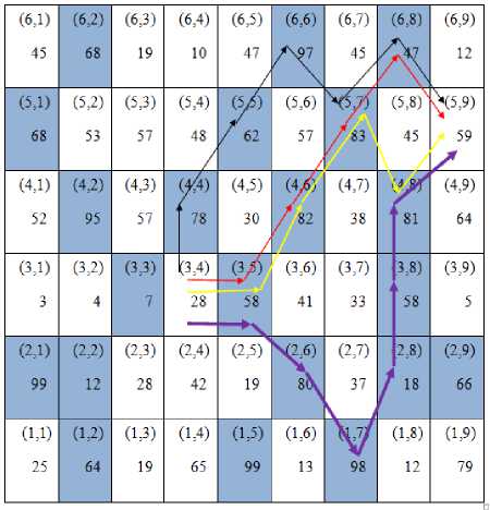
Fig 7: Routing protocol in GAFBone

For instance, we suppose a grid with the coordinates (3,4) transmits a query message to the node which is located at (5,9). There are four different links between the mentioned grids. The table II shows the value of α parameter in each stage, and the final quantity of this parameter. According to the table it is clear that the yellow path has a priority over all other connections.

Table 2. Different routes based on αlpha parameter

	15.6+15 2+312+41.5+33.5=137
	13.18+37.2+41.5+33.5=125.45
	13.18+ 37.2+41.5+57.8 =149.6
	13.18 +19+22 2+5.8+26.3 +57.8=144.28

V.    Simulations and results

We simulated the GAFBone in MATLAB [19]. We consider the deployment area as a square, and then partitioned it into equal grid cells with different size of side. For implementing three phases of this algorithm, the whole field and the grids considered as a matrix and elements of the matrix, respectively. Fig. 8 depicts two examples of running this algorithm. One of them is a region with 15 *15 grids, and the other one is 24*24 cells. The parts (a) in the figures show the amount of energy before applying the GAFBone. The highest rank grids in terms of energy show with white color, the lowest ones are being seen in black color, and the energy of other grids is in grayscale. After using the proposed algorithm, the parts (b) of figures will be achieved. In these pictures the black color represented as sleep grids. By comparing two parts (a) and (b) it can be seen that, the white grids are remained constant approximately, which means this algorithm uses high power nodes for routing packets, and turns off unnecessary nodes.

The table III considers the 100 * 100m area which divided into grids by use of GAF algorithm. As mentioned before, we suppose the number of rows and columns are multiples of three. Thus, the GAFBone simulated for eight different partitioning schemes from (6*6) to (27*27). By decreasing of grid size the total number of grids will be risen, therefore it takes long time to complete the GAFBone algorithm. On the other hand, the maximum range of frequency will be declined which causes to reducing the power consumption. The Maximum value of radio frequency depends on the grid size, and calculated based on the maximum distance between two adjacent nodes in 3*3 neighborhoods. According to Fig. 9 it equals to 2√2 г .

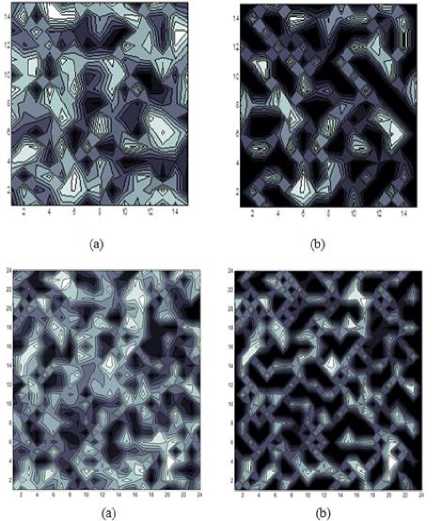
Fig 8: Energy Map of (15*15) and (24*24) grids.

(a) Before applying GAFBone (b) After applying GAFBone

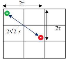
Fig 9: Calculation of maximum frequency range

Although GAFBone results to decrease the number of active nodes without any deficiency in routing packets, constructing this backbone consumes energy which cannot be ignored. The last column of table III shows the percentage of power consumption for GAFBone. For calculating these statistics, we suppose the algorithm consumes one unit power for each comparison of energy supply of neighbors’ grids. Therefore, after each comparison one unit subtracted from the total power of the network before GAFBone has been started. Afterward, the whole power before beginning GAFBone divides by a result of energy reduction. The coefficient of the division is taken as the percentage of energy consumption of the proposed backbone algorithm.

Table 3. Characteristics of different partitioning schemes for GAFBone

Rate of partitioning area	Grid Size (r)	Max Frequency Range	Total Grids	BB Grids (On Grids)	Percentage of Active Grids	Percentage of Energy consumption for GAFBone Construction
6*6	16.6	46.4	36	12	33.3%	2.4%
9*9	11.1	31	81	39	48.1%	2.4%
12* 12	8.3	23.2	144	64	44.4%	2.7%
15* 15	6.6	18.4	225	103	45.7%	2.9%
18* 18	5.5	15.4	324	154	47.5%	2.9%
21 *21	4.7	13.1	441	212	48.0%	3.1%
24*24	4.1	11.4	576	272	47.2%	3.2%
27*27	3.7	10.3	729	340	46.6%	3.2%

VI.    Conclusions

In this paper, we proposed GAFBone which is a new backbone construction for GAF routing protocol. GAFBone is a distributed algorithm which makes an effort to diminish active grids while the network maintains its connectivity. This approach considers 3*3 neighborhoods, and by the use of central grid ensures that this vicinity can communicate with each other, then generalizes this idea into the whole network. In this scheme, we consider an assumption that the number of rows and columns are multiples of three; also there is the possibility to reduce more redundant active grids. Hence, ignoring this assumption, and finding inessential awake nodes included in future work.