Gait Recognition for Human Identification Using Fourier Descriptor and Anatomical Landmarks

Published Online January 2015 in MECS

Physical biometric traits like face, fingerprint and iris are typically used in applications to identify human beings. Recent research has demonstrated the possible ancillary information such as gender, height, weight, age and ethnicity to improve the recognition accuracy of biometric systems.

Gait is the systematic study of human walking styles and in due course of time it has drawn lots of attention of people. For example, Borelli [1], an Italian Scientist, in 17th Century, pioneered the animal gait movement (locomotion). Braune [2] in the year of 1890 did a tremendous work on biomechanics using lithographic cross section of human body.

Human gait shows distinct characteristic of person and also the walker’s physical and psychological status. Research on gait analysis can be expressed on medical perspective. Murray [3] used gait to classify the pathologically abnormal patients into different group for appropriate treatment. This classification was achieved by comparing a patients’ gait patterns with normal gait patterns obtained from a control group.

Because of its potential for human identification at distance human gait recognition is developing tremendously in terms of computer vision research. Since it is difficult to identify person from pictures taken from a distance by some other biometric, gait has made it possible by taking a person’s image in different sequences.

Different methods and approaches have been proposed to identify human beings throughout more than a decade.

Jiwen Lu and Erhu Zhang [4] proposed a method for gait recognition on the basis of human silhouettes using multiple feature representations and Independent Component Analysis (ICA).

Considering multiple features and fusing them and classify on the basis of Genetic Fuzzy Support Vector Machine (GFSVM), good recognition result has been obtained. In their proposed method they have considered three view fusions, i.e. perpendicularly, along and oblique with the direction of human walking.

Lee and et. al [5] proposed a method that attempted to divide the human body into components that are treated separately . In their work, a silhouette is represented by seven ellipses and by using Fourier transform they extract features from the change in magnitude and phase components and discrimination power from these components during walking of the subject. These features were used for person identification and gender classification and for relatively small dataset it produced good results.

Cunado et al. [6] proposed an approach where gait signature is extracted from a sequence of walking using the Fourier series to represent the motion of the upper leg. K-nearest neighbor classification rule was applied to the Fourier components of the motion of the upper leg. By the phase-weighted Fourier magnitude information when compared to the usage of the magnitude information enhanced classification rate is obtained.

By the analysis of image sequence, visual analysis of human motion [7] [8] detection, tracking and identification of any object has become possible. Over the past few years, the combination of biometrics and human motion has become a popular research. The vision based human identification at a distance has gained wider interest from the computer vision community. For automated person identification system in visual surveillance and monitoring application in security purpose such as banks, parking lots, airports and railway station etc this interest is strongly motivated.

Contributions of this Paper

Here, Fourier Descriptor has been applied to for shape extraction and analytical landmarks have been considered for control point selection.

Different angles, like angle created between the Centre of Mass, Knee and Ankle (CKA), angle created between Centre of Mass, Wrist and knee (CWK) have been measured along with angles i.e., DCC and Distances between the Centre of mass and the Control points i.e. ABLC have been calculated.

Section 2 describes feature extraction technique,

Experiments conducted for this work along with results are described in section 3 and section 4 concludes this work.

• II.    Feature Extraction

• 2.1    Object extraction

For any kind of recognition concern the feature extraction is a vital and major part. Before approaching the feature extraction stage, it is needed to collect the video sequences of different persons and dividing the video sequences in fixed time interval the static images of every moment of walk is taken in such a way that the entire gait movement cycle can be obtained and by the following procedures they are converted to binarized silhouette images to simplify our work. Features are extraction from these silhouettes has been described below.

Considering that the object is moving and camera is static, the video sequences have been taken and the snapshots have been taken in such a time interval that the gait signatures are fully realized.

The first and foremost thing is to subtract the background from the entire image to have the foreground object or the subject under concern.

Based on background subtraction and silhouette correlation the extraction and tracking of moving silhouettes from the background in each image-frame the detection and tracking algorithm is used.

By LMedS (Least Median of Square) [9] method background image can be generated from a small portion of image sequence.

Siegel's estimator [9] for LMedS is defined as follows:

For any m observations (x , y ), …., (x ,y ) which i1 i1 im im determine a unique parameter vector, the jth coordinate of this vector, denoted by θ (i ,......., i ). The repeated median is then defined coordinate-wise as

θ _j = med (…..( med ( med θ _j (i₁ ,..,i m )))…)……(1) ⁱ 1                     ⁱ p - 1           ⁱ m

Let I represent a sequence including N images. The background β(x,y) can be computed as given in [9], by

β(x,y)= min { med f (I^f(x,y)–b)²}………….(2) b

Where, b=background brightness value at pixel location (x, y). med= median value f=frame index from 1 to N

It is difficult to select suitable threshold for binarization since the brightness of the entire sequence of gait cycle may not be same throughout, i.e. it may vary on time, and the brightness change can be obtained through differencing between the background and the current image and especially in case of low contrast image as the brightness change is too low to distinguish between object from noise. This problem can be solved by the following function which has been used to perform differencing [10] indirectly

• =-    ( α ( x , y ) + 1)( β ( x , y ) + 1) 2 ( η - α ( x , y ))( η - β ( x , y ))

m ( α , β ) = 1 -                           .

• ( α ( x , y ) + 1) + ( β ( x , y ) + 1) ( η - α ( x , y )) + ( η - β ( x , y ))

• 2.2    Fourier Descriptor for shape extraction-

• The Fourier descriptor helps in describing the boundary of the object effectively. The boundary point k can be expressed as complex function

Where, α (x,y) is the brightness of current image at pixel position (x,y), β (x,y) is the background at pixel position (x,y) of current image, η is the maximum intensity value i.e. for gray scale it is 255, 0<= α (x,y), β (x,y)<= η and 0<= m ( α , β )<1.

Erosion and dilation operations are generally used to fill small holes inside the extracted silhouette to remove noise as much as possible

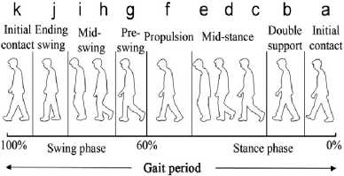
Fig.1. The specific phases of gait period (a)–(k): stance phase (a)–(f) comprising about 60% of the gait period; and swing phase (g)–(j)

There are two phases of walking, the Stance phase and Swing phase. Swing phase occurs when one leg will be in air and in the Stance phase both the legs will be on ground. It has been observed that 60% of walk is in Swing phase and 40% is in Stance phase. There are ten sub-phases in between Swing and Stance which can be seen from the figure1.

S(k)=X(k)+jY(k)               (4)

The procedure of obtaining Fourier descriptor [11] is illustrated as follows:

• i)    Take N digital points of the boundary, where N represents the length of the closed curve.

• ii)    Apply the Fourier transform to the boundary points.

j 2 Π ux

₁ N - 1          _N

S(u)=       T ( k ) e     ,for k=0,1,2,…N-1    (5)

N k = 0

• iii)    The inverse transform can be applied to obtain the original points

j 2 Π ux

₁ N - 1          _N

T(k)=       S ( u ) e      ,for u =0,,1,2,…N-1  (6)

N u = 0

The coefficients S(u) are called Fourier descriptors. They represent the discrete contour of a shape in the Fourier domain.

Scale invariance of Fourier descriptors can be achieved by dividing all Fourier descriptors by the magnitude of the second Fourier descriptor (i.e. I S(1) I ); thus the scale invariant vector (S(k)) may be written as S(k)=

S ( k )

I S (1) I

On the other hand, the rotation invariance may be achieved by keeping the shape of the original contour representable via the rotation invariant Fourier descriptors, the orientation of the basic ellipse is used, which is defined by the Fourier descriptors s(1)= r 1 e^j ϕ ¹ and s(-1)=r -1 e^j ϕ ^-1 , as

T e (n)=s(-1)e^-j2 π ^n/N+s(1)e ^j2 π ^n/N .............(8)

After a number of transformations, equation(8) can be written as

_T(n)=ej( ϕ _{- 1}+ ϕ ₁)/2_{[r e}-j( ϕ ^∧ +2 π n/N) _{+ r e}j( ϕ ^∧ +2 π n/N)_]

Where ϕ ^∧ = ( ϕ 1 - ϕ - 1 ⁾/2).

Equation (9) shows the rotation ϕ e of the basic ellipse by

ϕ e = ( ^ϕ - 1 + ^ϕ 1 )/2……………(10)

An ambiguity of π radians can be observed by using the orientation of the basic ellipse. Thus the rotation invariant Fourier descriptors are only rotation invariant modulo a rotation by π radians.

Moreover, The position of the starting point may be normalised by subtracting the phase of the second Fourier descriptor weighted by k from the phase of all Fourier descriptors, i.e.

S(k)=S(k)e^-j ϕ 1 ^k ………… ...(11)

• 2.3    Center of Mass Detection

A normalized point or center of mass is needed that will be significant point in terms of the contour points of that subject. A rectangle which encloses only the contour of the subject, called bounding rectangle is considered to crop the image according to the perimeter and resized to a fixed height while preserving the aspect ratio (i.e., ratio of silhouette width to its height) using bilinear interpolation.

The resized contour is then copied to a destination image of fixed size by coinciding its centre-of-mass with the centre of the destination image to make it translation invariant.

A 2D Cartesian moment is a gross characteristic of the contour computed by integrating over all of the pixels of the contour. The (r , s ) moment of a contour can be defined as

n mr ,s=∑I(x,y)xrys          (12)

i = 1

Here r is the x -order and s is the y -order, whereby order means the power to which the corresponding component is taken in the sum. The 2D Cartesian coordinate of center of mass C (x c , y c ) is the ratio of the 1^st order and 0^th order of contour moment [12].

x c =m 10 /m 00 ,  y c =m 01 /m 00 ................. (13)

m00 moment is the length in pixels of the contours when both r and s both are zero.

m10 and m01 denotes moment of x and y component.

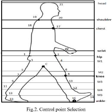
• 2.4    Control point selection

Selection of control points is very important and imperative in our work, since these points signify the gait characteristics of a subject under surveillance, to be extracted. Anatomical landmarks have been considered on the different locations of the human body as a fraction of subject’s height (H). From the concept of anatomical studies [13] the positions of ankle (Ak), knee (kn), Wrist(Wr), hip (Hp), chest (Ch), shoulder (Sl) and head (Hd) are estimated vertically as a fraction of the body height (measured as vertical height of the bounding rectangle enclosing the subject’s silhouette contour) as 0.039H, 0.285H,0.485H, 0.530H, 0.720H, 0.818H and 0.870H measured from the bottom of the subject i.e. maximum y coordinate level. The control points of the contour have been considered from these points, are treated as anatomical landmarks.

Now to have all the control points with the help of anatomical landmark points the following algorithm has been illustrated.

Algorithm 1:

Input: The boundary point set BP of the subject in the bounding rectangle.

Output: Generate the control points 1-21.

• i)    The boundary point set BP={b_k}, k is number of boundary points. Each b_k has x and y coordinate named x_k, y_k.

• ii)    Perpendicular distances ∀ b_k (x_k, y_k) from maximum y coordinate(say y m ) (bottom level) has been found out. Let it be D k ,

D k ={y k -y m | ∀ k}               (14)

• iii)    The perpendicular distances of anatomical points Ak, Kn, Hp,Wr, Ch, Sl, Hd from y m as d Ak , d Kn , d Hp , d wr , d_Ch, d_Sl, d_Hd have been calculated as the vertical height of the bounding rectangle.

• iv)    Comparing these distances (d Ak , d Kn , d Hp , d Ch , d Sl , d Hd) with D k set, the index points have been found out.

• v)    These index points are compared with BP i (index of boundary point set)(1 ≤ i ≤ k)

From the matched index value of BPi’s the corresponding x and y coordinates of corresponding anatomical points are extracted.

• vi)    From one anatomical landmark point the opposite coordinate can be found out from the set BP. (e.g. the point on hip marked as 2 and the opposite is marked as 1). From a landmark, comparing the y coordinate point with all corresponding x coordinate points from the set BP, the minimum x coordinate point will be taken from the set BP, this (x, y) point denotes opposite point. Similar way points 7, 15, 18, 19 have been found out.

• 2.5    Leg Rise from Ground (LRFG)

The middle y coordinate points between centre of mass and hip (say M1), knee and center of mass (say M2), knee and ankle (say M4), knee and M4 (say M3), ankle and M4 (say M5) have been considered and corresponding x coordinate value have been extracted from the set BP and from the step (vi) the opposite points are also obtained. In this way all the control points (1-22) have been found out and kept in set named CntP serially.

From the silhouette images the control points thus extracted as described in the algorithm in section 2.4, so to get more information about the images in the sequences in feature extraction, the measure, LRFG has to be determined. Maximum y co-ordinate point of the bounding rectangle is marked as the ground level. Now, using the index of this point from the set BP, the corresponding x co-ordinate is determined. The vertical positions of knee (Kn) are estimated as described by the section 2.4. The height is calculated by the Euclidean distance between head point and the perpendicular point B (shown in Fig.3). The algorithm for finding the leg rise is given below:

Algorithm 2: Calculation of LRFG measure.

Input: Boundary points set BP.

Output: Maximum normalized leg rise distance from horizontal line of the bounding rectangle.

Step1. A horizontal line which is nothing but the bottom level of the bounding rectangle has been considered.

Step2. Minimum x Co-ordinate has been found out from the boundary point set BP by

X min =min(x)              (15)

Where min denotes minimum value and the corresponding y coordinate has been taken from BP and this point denotes the heel point (A).

Step3. Perpendicular line has been drawn from A to C (C is the point considered by maximum y coordinate and minimum x coordinate respectively). The distance from the heel point A to the perpendicular point C is denoted by PER

Step4. Since the minimum y coordinate point has been treated as head point, corresponding x coordinated has been found out from the set BP. Draw a perpendicular line from head point to the horizontal line point B. Find the Euclidean distance from the point A to point B, denoted by AB.

Step5. Check whether the distances AB and AC is less than the distance between knee point (k) to Horizontal line, if so, it will be treated as a valid LRFG distance.

Step6. Normalized leg rise (LRFG) is considered by finding the ratio of (PER: AB).

Step7. The maximum normalized leg rise distance among all the stances in a sequence will be taken into the dataset.

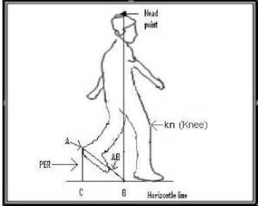
Fig.3. Leg Rise From Ground (LRFG).

• 2.6    Distance between Centre of Mass to Control points (DCC)

• 2.7    Angles created between the legs with the Centre of Mass (ABLC)

• 2.8    Angles created between the Centre of Mass Knee and Ankle with the (CKA)

From the silhouette boundary images the anatomical landmark points or control points have been found out as described in the section 2.4. The centre of mass (C(xc,yc)) of the object has been described in section 2.3 in equation (13) has been calculated. Now, the Euclidean distances from the centre of mass to the anatomical points of the objects are measured. The distances have been calculated considering the points C-2,C-3,C-6,C-7,C-9,C-12,C-13,C-16,C-17,C-19,C-21which is shown by the figure below:

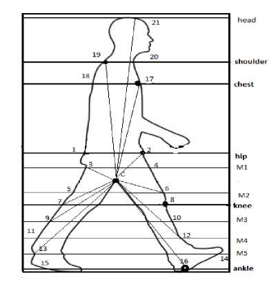
Fig.4. Distance from Centre of Mass to Control Points (DCC)

Another measure ABLC which finds out the angles created between the control points with the centre of mass. The angles between the control points with the centre of mass on the lower half of the centre of mass can be determined by [19] and the following angle have been calculated ∠ Cnt 7 C Cnt 6 , ∠ Cnt 5 C Cnt 8 , ∠ Cnt 10 C Cnt 11 , ∠ Cnt 12 C Cnt 13 , ∠ Cnt 14 C Cnt 15 , ∠ Cnt 5 C Cnt 16 , ∠ Cnt 8 C Cnt 13 For the upper half i.e above C, the angles ∠ Cnt 2 C Cnt 3 , ∠ Cnt 17 C Cnt 19 have been found out. From the fig.5 it can be easily realized.

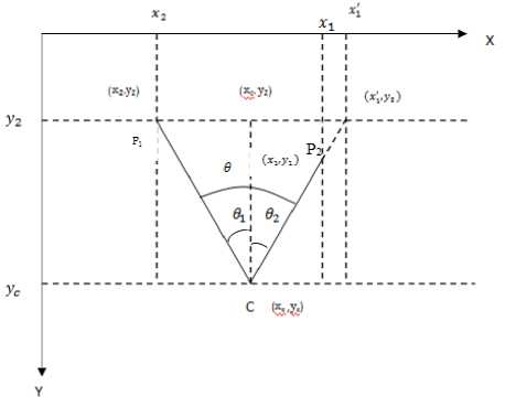
Fig.5. Angles created between control points of upper portion of point C to the C.

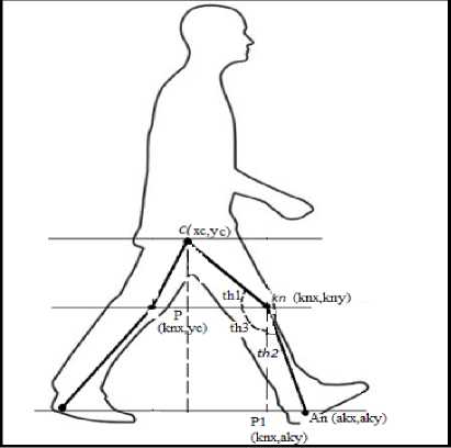
Fig.6. Angles created between the Centre of Mass, Knee and Ankle with the (CKA)

The angle created with centre of mass, leading knee point and leading ankle can be found out. A Perpendicular line is drawn from Centre Of Mass(C) to bottom level and a horizontal line through the knee point (kn). The intersection point between these points is P

(knx,yc). Now the angle created between Centre of mass knee point and P i.e. Z C kn p xc - knx ,h',an  yc   b,..................(15)

Another Perpendicular line is drawn from knee point to the ground level. Now since this line is perpendicular to the horizontal line via points P and knee, the angle th3 is obviously 900. The perpendicular line from knee point to the bottom level intersect the horizontal line drawn via ankle point An at P1 (knx, aky).The angle created between ankle, knee and P1 i.e Z An kn P1 can be written as akx - knx th2=tan kny - aky         (16)

passes through wrist point wr and the perpendicular line from C intersect that line at C1(cx, wry).Another horizontal line is drawn from knee point which cut the perpendicular line from wr at K(wrx, kny) Now the Z C1 wr C can be calculated as yc — wry th5=tan-1 wrx—xc the angle Z kn wr K can be calculated as knx - wrx th4=tan-1 wry - kny since Z C1 wr K is a right angle the angle Z C wr K can be found out by th6= 900-(th4+th5)(21)

Now the angle created between Centre of Mass, knee and ankle can be written as th=th1+th2+th3              (17)

When the legs will not far away to each other or in case of swing phase the legs are not so stretched, in that case the x coordinate akx of ankle point will be less than knee point knx.

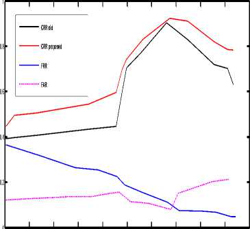
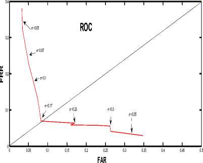
So, if akx>knx the angle th can be found out from the equation (17), otherwise i.e. for akx

• 2.9    Angles created between Centre of Mass, Wrist and knee (CWK)

Fig.7. Angles created between Centre of Mass, Wrist and knee (CWK)

To find out the angles between the Centre of mass, Wrist (which is measured from anatomical landmarks by 0.485H) and knee point the following procedure is followed. Draw perpendicular line from the wrist to any point on leg (say B) and draw a horizontal line which

• III.    Experiment And Results

• 3.1    Mahalanobish Distance

The experiment has been conducted by using CASIA-C dataset [14]. Here 21 control points have been considered and out of these 11 different angles and 11 different distances and 1 LRFG for each gait sequence or in total 23 parameters have been calculated and treating each column as a parameter value in the extracted feature set. If in a sequence there are n images then for a person’s each gait sequence, the training dataset consists of 23x n matrices.

In this work, it is assumed that these parameters follow Normal Distribution. Let, X ,X ,...., X are the random variables corresponding to the parameters. So the joint probability density function (PDF) of these variates is multinormal. Thus, for each sequence, the PDF is Multinormal with different population parameter values, such as population mean vector and population variancecovariance matrix.

For two sample matrices or for two gait sequence of order 23 x n to determine whether they are from same person or not, sample version of Mahalanobis distance [15] has been used.

For sample training and testing vectors, let, ^ and ^₂ be the mean vectors respectively (the mean vectors are vectors of column wise mean values) and S₁ and S₂ are the sample variance-covariance matrices of the training and testing data respectively.

Let,

S = (S + S₂ )/2           (22)

Mahalanobis distance statistic says

D²= (^1-^2) TS-1(M"M2)     (23)

If the value of D²is less than or equal to some threshold value, then it can be inferred that the gait sequence is of same person, otherwise it is not in the database.

• 3.2.    Threshold value

For threshold calculation k number of gait sequences of the same person have been considered. In each case, the D²values have been calculated. Let, these D²values are D²1 , D²2, , D²k .

Now,

D 21 k = !(D 21 + D \ ++ D2 k)     (24)

k

In this way, for p persons and k sequences each D²1k , D²2k , ,D²pk have been calculated and an average value is considered i.e.

D²avg = -(D²i k + D²2 k +.....+ D²pk)    (25)

p

D²avg + <7 , has been chosen to be the threshold value where, <7 is the precision value defined by

7 = !((D²avg - D²1 _k)²+.....+ (D²avg - D²pk)²)^{1/2   (26)}

p

In this experiment, gait sequences of 100 persons have been considered and corresponding feature set of gait sequences have been created. The vectors for each person and for each sequence of the order of 23 X 25(considering in each sequence there are 25 images). Since, 3 sequences of a person have been taken, the feature vector would be in the form of three matrices having dimension 23 X 25 and D² values are calculated with sequence 1-2, 1-3 and 2-3 and calculate D²_avg and the precision value by applying the equations (25) and (26).

For individual persons the D2 values i.e. D21 ,D22 ,....., D2k (where k is the sequence number, in this case k = 3 have been considered) have been calculated. And for the 100 persons the D2avg has been calculated and it is 0.32348.

• 3.3.    Training and Testing Algorithm

Algorithm-3: Training

Input: Image sequences of different persons. Output: Training dataset and threshold.

Step 1. Create Database of Silhouette images of different persons.

Step 2. Step2-for each pair wise gait sequence of the same person do the following

• a.    Find out the boundary of each subject in each image using Fourier Descriptor.

• b.    From the concept of analytical landmarks find out the control points by algorithm 1.

• c.    Calculate the Centre Of Mass (C) as described in section 2.3.

• d.    Create the feature set by following components-

• i)    The Leg Rise from the ground (LRFG). ii)    The Euclidean Distance between the Centre of Mass and the control points (ABLC). iii)    The Control angle between the Centre of Mass and the control points (DCC). iv)    angles created between the Centre of Mass, Knee and Ankle with the (CKA), v)    angles created between Centre of Mass, Wrist, knee (CWK),

• e.    Compute the pair wise Mahalanobish-distance for the gait sequences of the same person and store these values for each person.

• f.    Compute threshold value using the procedure described in section 3.2

Algorithm-4: Testing

Input: Unknown Gait Sequence

Output: Match or No Match

Step 3. Take a gait sequence of an unknown person.

Step 4. Extract features by the procedure described in step2- (a)-(d) of algorithm-3.

Step 5. Compute Mahalanobish-distance between the testing data and each training sequence data with predefined threshold value to test for matching.

The precision value is obtained experimentally. A good response of recognition depends on this precision value. This value can be positive or negative. It has been depicted in the figure- 8. The response of the false rejection rate (FRR), false acceptance rate (FAR) and the correct recognition rate (CRR) in accordance with value of ±σ. It has been found out that correct recognition rate was 91% in our old method but in this proposed approach the CCR is 92.3% and both the FAR and FRR is 8% if σ = 0.17.i.e for the threshold value D2avg + 7 =0.49348 =0.5

No. of Persons

Fig.7. The D²1k , D²2k ,.....,D²pk values corresponding to 100

persons are mapped in this figure

-0.5             -0.4             -0.3             -0.2             -0.1                0               0.1

±σ

0.2              0.3              0.4              0.5

Fig.8. Plot with ±σ and the Recognition Rate

The fig.8 shows the recognition rates for both the +ve and –ve values of σ. It shows below the zero value of σ i.e. in the –ve direction the response of CRR and FRR, FAR is not appreciable compared to the +ve direction and when σ=+0.17, CRR becomes maximum i.e. 92.3% and considering the trade of between FAR; FRR the value can be taken at 0.079 of RR i.e.7.9%. Comparing the two CRR curves i.e. black and red (black shows our old method [19] and red shows proposed approach), it can be seen that CRR of our proposed approach gives us better correct recognition rate.

Fig.9. From the ROC curve the ERR value is 0.79 for σ = 0.17 i.e. at this point FAR=FRR.

Fig 9 shows ROC for different value of σ but when σ=0.17 maximum recognition rate is obtained.

Table 1. Different Recognition Parameters

Person	Correct recognition	Correct rejection rate	False acceptance rate	False rejection rate
100	92.3%	92%	7.9%	8%

To examine the performance of the proposed algorithm, comparative experiments have been conducted which is shown in table-2. From Table-2, it is clear that the method, proposed here, has shown significant improvement in performance as compared to other recent methods for same database.

Table 2. Comparison of different approaches with our methods

Method	Database	Recognition Rate
MijG(x,y)+ACDA [16]	CASIA-C	34.7%
GEI [17]	CASIA-C	74%
2DLPP[18]	CASIA-C	88.9%
Our Old method [19 ]	CASIA-C	91%
Proposed Method	CASIA-C	92.3%

• IV.    Conclusion

This paper focuses on the idea of using Fourier descriptor based shape extraction on silhouette-based gait characteristics. Gait has a rich potential as a biometric for recognition though it is sensitive to various covariate conditions, which are circumstantial and physical conditions that can affect either gait itself or the extracted gait features. Example of these conditions includes carrying condition like backpack, briefcase, handbag, etc., view angle, speed and shoe-wear type etc. or physical conditions like pregnancy, injury on legs etc. Our technique is very good in terms recognition accuracy but here only lateral view with movement been considered, so there is a good scope to extend this technique on different view angle between camera and object.

Acknowledgement

The authors would like to thank Mr. Hongyu Liang for providing the database of the silhouettes named “CASIA Human Gait Database” collected by Institute of Automation, Chinese Academy Of sciences. Their thanks also go to those who have contributed to the establishment of the CASIA database [14].

This work has been carried out at “Center for Machine Learning and Intelligence” under computer science and engineering department of Supreme Knowledge Foundation Group of Institutions (SKFGI), Mankundu, Hooghly, West Bengal, India.