General software/hardware approach in acceleration of quantum computing and classically efficient quantum algorithm simulation

Author: Barchatova Irina, Rizzotto Gian Giovanni, Porto Massimo, Ulyanov Sergey
Journal: Сетевое научное издание «Системный анализ в науке и образовании» @journal-sanse
Article in issue: 3, 2014.
Free access
This article describes how to build a classical hardware (HW) device, which accelerates the simulation of QA on classical computer. The usual approach for so doing consists in the simulation of the either QAs and their underlying quantum systems. The main aim of this article is not to work on real quantum HW (as quantum dots, ion traps, NMR etc.) but to take quantum computing as a computation paradigm (alternative to classical computing and soft computing).
Quantum algorithm, software simulation, hardware of quantum computing acceleration
Short address: https://sciup.org/14122612
IDR: 14122612
Общий подход к проектированию программного и аппаратного обеспечения для ускорения квантовых вычислений и классически эффективное моделирование квантовых алгоритмов
В данной статье рассматривается вопрос построения классической аппаратной поддержки, позволяющей ускорять моделирование квантовых алгоритмов на классическом компьютере. Обычный подход к решению данной проблемы заключается в моделировании непосредственно квантового алгоритма с последующей реализацией в соответствующей квантовой системе. Целью данной статьи является реализация квантовых вычислений как вычислительной парадигмы (альтернатива классических и мягких вычислений) без использования квантовой аппаратной части (например, квантовых точек, ионных ловушек, ядерных магнитных резонансов и т.д.).
Text of the scientific article General software/hardware approach in acceleration of quantum computing and classically efficient quantum algorithm simulation
ОБЩИЙ ПОДХОД К ПРОЕКТИРОВАНИЮ ПРОГРАММНОГО И АППАРАТНОГО ОБЕСПЕЧЕНИЯ ДЛЯ УСКОРЕНИЯ КВАНТОВЫХ ВЫЧИСЛЕНИЙ И КЛАССИЧЕСКИ
ЭФФЕКТИВНОЕ МОДЕЛИРОВАНИЕ КВАНТ ОВЫХ АЛГОРИТМОВ
Бархатова Ирина Александровна1, Ризотто Джиани2, Порто Массимо3, Ульянов Сергей Викторович4
1Аспирант;
ГБОУ ВО «Международный Университет природы, общества и человека «Дубна»,
Институт системного анализа и управления;
141980, Московская обл., г. Дубна, ул. Университетская, 19;
2Доктор наук, профессор;
ST Microelectronics;
20041, Италия, Agrate Brianza, Via C. Olivetti, 2;
3Доктор наук, профессор;
ST Microelectronics;
20041, Италия, Agrate Brianza, Via C. Olivetti, 2.
-
4Доктор наук, профессор;
Факультет механики и технической кибернетики (интеллектуальные системы), Университет передачи информации;
1-5-1, Япония, Токио, Chofu, Chofugaoka ,182;
-
8Доктор физико-математических наук, профессор;
ГБОУ ВО «Международный Университет природы, общества и человека «Дубна»,
Институт системного анализа и управления;
141980, Московская обл., г. Дубна, ул. Университетская, 19;
The general approach for quantum algorithm (QA) simulation on classical computer is introduced. Efficient fast algorithm and corresponding SW for simulation of Grover's quantum search algorithm (QSA) in large unsorted database is presented. Comparison with common QA simulation approach is demonstrated. Hardware (HW) design method of main quantum operators that are used in simulation of QA. Grover’s QSA as Benchmark of HW design method application is considered. This approach demonstrates the possibility of classical efficient simulation of QA gates (QAG) [1 – 5].
Quantum computing is not only a beautiful way of exploiting HW devices governed by quantum mechanics, but also a new approach for information processing which may (and is) interesting and useful. The ideas introduced by quantum computing, like the use of reversible operators, have applications even without the disposability of real quantum computer. In fact in the rest of this report the new methodologies, which hybridize quantum computing and soft computing (referred to as Quantum Soft Computing methodologies) are introduced.
These new methodologies widen the range of applicability of soft computing techniques, keeping their actual advantages. Since we are interested in applying the quantum computation paradigm, our approach consists first in the analysis of the input-output relations of each block and then in the simulation of these relations. In particular, we present a new circuit implementation of QSA with information criteria (minimum of Shannon entropy) for search termination process that is the background for optimisation of control processes. We focus our attention on superposition , entanglement , and interference quantum operators (there are the fundamental quantum operations of QSA) and propose a new HW accelerator structure for Grover's QSA.
All the proposed HW architectures are modular in the sense that they can be generalized by adding similar parts according to the desired number of q-bits; furthermore we don’t use multipliers and, by utilizing logic gate in an analogical scheme, we reduce the number of operation and component, providing a substantial increase in speed-up of computation.
-
1.1. Fast algorithm and HW design for efficient computational intelligence of main quantum algorithm operators on classical computer
Quantum algorithms (QA) demonstrate great efficiency in many practical tasks such as factorization of large integer numbers, where classical algorithms are failing or dramatically ineffective. Practical application is still away due to lack of the physical HW implementation of quantum computers.
We describe design method of main quantum operators and hardware (HW) implementation of QAG for fast search in large database and related topics concerning the control of a process, including search-of-minima intelligent operations . This method is very useful for minimum efforts of searching among a set of values and in particular is the first step for the realization of a HW control systems exploiting artificial intelligence in order to fuzzy control in a robust way a non-linear process or in order to efficient search in a database. The presented HW performs all the functional steps of a Grover QSA (This algorithm and its modifications are described in Chapter 1 and 4). By suitable changes of traditional matrices approach, a modular n -q-bit-hybrid structure is realized in order to prove the usefulness of iterations of the gate, which provide a higher probability of exact solution finding. A minimum-entropy based method is adopted as a termination condition criterion and realized in a digital part together with display output. The possibility of providing an external clock signal for iteration management allows implementing a very fast Grover’s QSA, many times faster than the corresponding software (SW) realization, and less sensitive to q-bits improvement.
The difference between classical and QAs is following: problem solved by QA is coded in the structure of the quantum operators. Input to QA in this case is always the same. Output of QA says which problem was coded. In some sense you give a function to QA to analyze and QA returns its property as an answer. QA studies qualitative properties of the functions.
The core of any QA is a set of unitary quantum operators or quantum gates. In practical representation quantum gate is a unitary matrix with particular structure. The size of this matrix grows exponentially with the number of inputs, making it impossible to simulate QAs with more than 30 – 35 inputs on classical computer with von Neumann architecture.
In presented Chapter we are described a practical approach to simulate most of known QAs on classical computers. We demonstrate the results of the classical efficient simulation of the Grover’s QSA as a Benchmark of this approach and background for quantum soft computing and fuzzy control based on quantum genetic (evolutionary) algorithms and quantum neural network. The role of this approach in quantum soft computing and in fuzzy simulation is also discussed.
Let us consider a new design method of HW architecture and implementation for main quantum operators using as Benchmark Grover’s QSA and fast algorithm simulation of main quantum operators.
-
1.2. HW implementation of main quantum algorithm operators
It has been found a new method and circuit that implements the operations performed in second and third step of a QA (the so-called entanglement and interference operators), able to perform Grover interference without products.
The proposed circuit, which is one of the first HW realization of QA, is also the first one not based on matrices products but on functional relation between input and output vectors.
A general form of the entanglement output vector UF = G can be the following:
G = [ g1, g2> — > gi ,—, g 2 n+1], where g. = y. Ф f and yt is the general term of superposition transformed in a suitable binary value. 1+ 2
The so-called superposition vector is fixed if we choose as input the canonical base. In order to find a suitable input-output relation, some particular properties of matrix Dn ® I have to be taken in consideration. The generic element v i of V (that is our output in Eq. (2)) can be written as follows in function of g i :
vi =1
1 £
2 n -1 ^^ g g2.
- g i , for
i odd
j = 1
2 n
E g 2 j - g i ,
for
i even
j = 1
This fact allows a great reduction of the number of operation (and therefore of electronics components) and consequently a significant increase of computational speed.
According to the proposed high-level scheme, our circuit realization can be divided into two main parts:
-
1.3. Limitations of classical approaches: A new strategy of computation for entanglement and interference operators
Following classical approaches, it is quite evident that the number of q-bits of a QA could be very critical in terms of computational speed. In fact, it must be noted that the addition of only one q-bit implies that matrices dimension become double with respect to the previous configuration and the number of elements (and of products) increases exponentially.
Preparing the gate with n q-bits set to |0>, the output of superposition can be represented in the following way:
Y =[ y 1 y 2 …… y i …… y 2 n+1 ], (3)
where y i =(-1)i+1/2(n+1)/2. Therefore, the output Q of the whole quantum gate becomes
G = [(Dn ®I)• Uf]h • Y (4)
in which a sparing of operations can be noted.
However this is not sufficient, being most of the computational weight due to entanglement matrix U F and interference matrix D n ® I , which have to be iterated several times. Similarly to the case of superposition, a single-element approach is followed to find the functional relation existing between the output vector and the corresponding input. All the necessary operations can be therefore implemented via simple logical and analogue gates.
This fact will be explained in the following section.
-
1.4. A new design method for entanglement and interference
The most important problem in a software implementation of the algorithm is that some of the speed performances vanish due to the vector representation of q-bits and, above all, to tensor products of matrices, which spend a lot of time in order to be executed. Moreover, it must be remarked that larger databases need larger amount of products, especially in the interference block. To this aim an alternative method and the corresponding circuit for the operation entanglement and interference is proposed. It avoids the use of multipliers and, by utilizing only logic gates and OPAMPs, reduce the number of operation and components.
1.4.1. Entanglement method and circuit design
All the steps for entanglement circuit design are presented here. The case concerning two q-bits is analysed, being the case with more q-bits a simple extension of it. Let us suppose to consider a function f: {0,1} 2 ^ {0,1} having the following definition law:
Г f (01) = 1
[ f (.) = 0 elsewhere
Its graphics is depicted in Fig. 1.
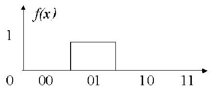
Figure 1. The definition of function f ( x )
According to the theory and design method, this function should be translated into an injective function F :{0,1} 3 ^ {0,1} 3 and therefore into U f in order to obtain the output of entanglement G=U f • Y.
The following method allows bypassing the use of F and UF providing directly the output vector. Since each element of the superposition output vector may assume a y or a –y value (where y depends only on the number of q-bit), Y can be easily transformed in a binary vector through the substitution yi ^ (yi +y)/2.
This fact allows performing exchange operations of entanglement in a simple way by using driven switches or XOR gates like in Fig. 2, in which a 2-q-bit case is represented. The values of f are taken as the second input in each couple of gate while all the elements of superposition vector are sent to the first ones. It can be noted that, if n is the number of q-bit, 2 n +1 components are needed instead of 22 n + 2, which is the number of elements of U F .
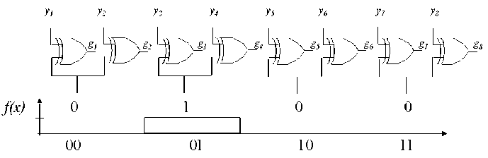
Figure 2. Circuit implementation of entanglement operator, 2 q-bit case
A general form of the entanglement output vector G can be the following:
G = [g1 g2 …… gi…… g2n+1], where gi = yi © fi+iNT(i -i)/2 and yi is the general term of superposition transformed in a suitable binary value.
In our example we have f 1 =0, f 2 =1, f 3 =0, f 4 = 0 and
1 11 11 111
22 22 22 22 22 22 2222
that in binary form becomes Y =[1 0 1 0 1 0 1 0]T. From previous considerations it can be found that G =[1 0 0 1 1 0 1 0]T or , by applying the reverse transformation
1 1 111 111
22 22 22 22 22 22 2222
1.4.2. Interference method and circuit design
A quite more difficult task is to deal with interference operator. In fact, differently from entanglement, in this case vectors are not composed by elements having only two possible values. Moreover, the presence of tensor products, whose number increases dramatically with the dimensions, constitutes a critical point at this step. In order to find a suitable input-output relation, some particular properties of matrix D n ® I have to be taken in consideration.
Odd columns (or rows, being D n ® I symmetric) have nonzero odd elements and even columns have nonzero even elements. This fact descends easily from the definition of tensor product.
If we except i th element of i th column (diagonal elements), the value of all nonzero elements is 1/2n-1. In the cited exceptions, these values are the same but decreased of 1.
Considering G the output vector of entanglement, the direct product V =( D n ® I ) G (output vector of interference) involves only a suitable weighted sum of its elements, being the value 1/2n-1 dependent only by the number n of q-bits.
From the above analysis, the generic element v i of V can be written as follows in function of g i :
v =1
n - 1
2 n
Z g2 j-1 - gi , for i odd j=1
n - 1
2 n
Z g 2 j — g i , for i even j = 1
This simple but powerful result has several consequences. Regarding the computational speed, a great improvement has been provided due to a smaller number of products (only one for each element of the output vector) and more precisely 2 n +1 against 4 n +1 of classical approach. Also additions are less than previously (2 n (2 n +1) instead of 4 n +1).
But the most important fact is that all these operation can be easily implemented in hardware with few operational amplifiers (2 n + 2). An example can be given in Figs 2 and 3 where a complete 2-q-bits Grover Quantum gate is depicted.
According to the above formulas, the pre-interference sum blocks perform separate sums of odd and even elements with a gain of 1/2 n - 1 (0.5 in this case). Each one of the eight OPAMPs outputs one element of the interference output vector. When the Grover search is finished, only two of them may assume values close to ±— U = ± 0.7071067 , denoting the position of searched element. With the same entanglement as in 2
the previous section, third and fourth OPAMPs (int3 and int4) must have nonzero values. This fact is confirmed by the particular of a PSPICE simulation depicted in Fig. 4 (707 mV against 0.1 mV of other outputs).
Part I: Base module. It implements a 3-q-bits system and it performs step-by-step calculation of output values. This part is divided in the following subparts:
|
a: Entanglement |
c: Interference |
|
b: Pre-Interference |
d: Modular interface |
Part II: Control module. It performs entropy evaluation in Eqs (3) and (1), vector storing for iterations and output visualization. This part also provides initial superposition of basis vectors |0> and |1>.
Entanglement operator composed by eight driven switches (see Fig. 6).
Referring to Fig. 7, the switches (MAX394) present in the circuit are only the odd ones. They receive the elements of initial superposed vector in couples (Vout1 and VN1, Vout2 and VN2…) and perform the exchange according to the signal coming from the encoder.
The output signals (O1, , O8) are the odd values of the entangled vector (even values are correspond ent opposite value). These values are summed and scaled (the scaling factor is ¼ in the case of three q-bits) by the OPAMP (see Fig. 7), which constitutes the pre-interference step.
The differences among this sum and each one of the elements are performed by the Interference block, whose structure is reported in Fig. 8.
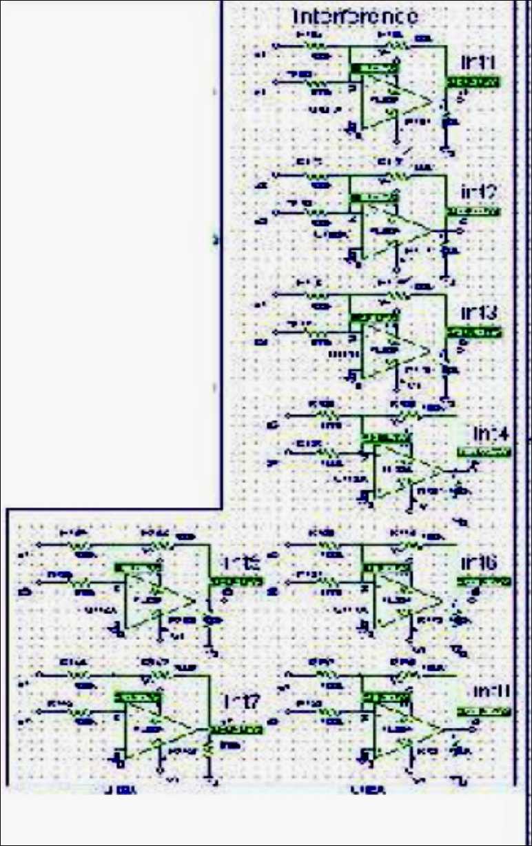
Figure 3. Interference gate implementation Grover’s QSA
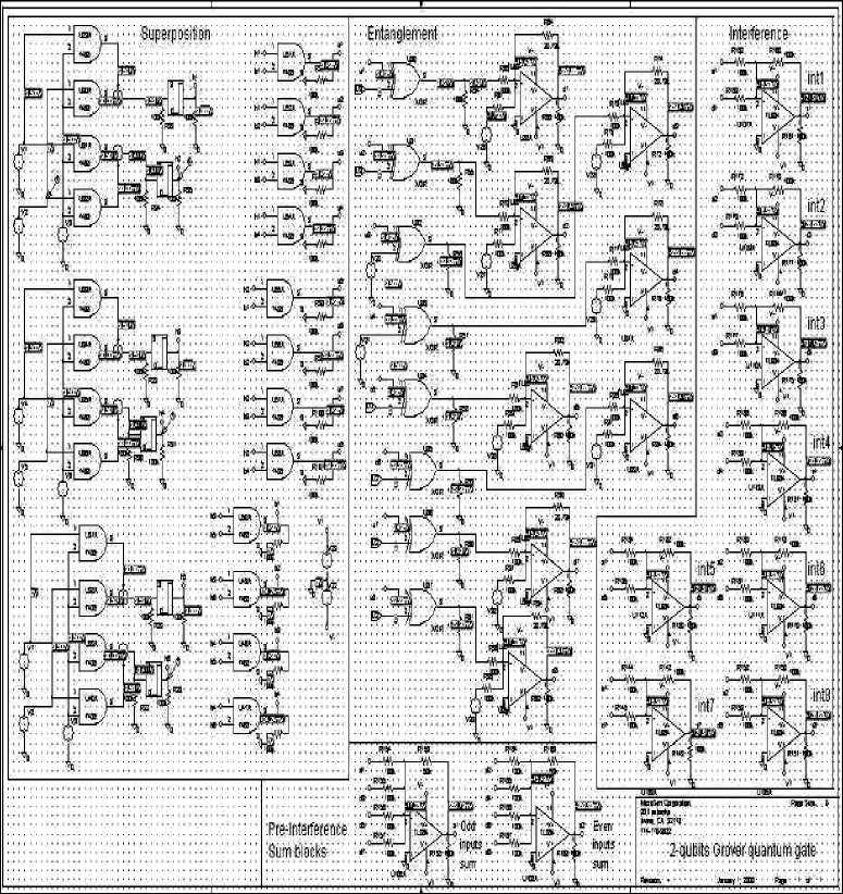
Figure 4. Grover’s QSA gate implementation (2-q-bits case)
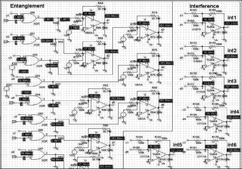
Figure 5. Circuit implementation for entanglement and interference operators in Grover’s QSA presented on the Fig. 4
|
IC1 1 |
Iff IN1 IN4 NO1 N04 COM1 COM4 NC1 NC4 V \A GND N.C. NC2 NC3 COM2 COM3 NO2 NO3 IN2 IN3 MAX394 |
20 LC4 |
|
"'//fl । 5 |
18 64 ^W4 |
|
|
-\\wUW jj — OSA |
||
|
13 63 |
||
|
^ *CC2 10 |
11 LC3"W3 |
|
US
|
ICS 1 |
IN1 IN4 NO1 N04 C0M1 COM4 NCI NC4 V V* GND N.C. NC2 NC3 COM2 COM3 NO2 NO3 IN2 IN3 |
2 0 l-CS |
|||
|
18 M |
|||||
|
и- |
—^^ |
||||
|
S^ute» 06 g |
13 67 ^™" |
||||
|
^*Й6 10 |
11 LC7^W |
||||
|
MAX394 |
|||||
Figure 6. Entanglement circuit
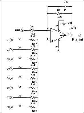
Figure 7. Pre-interference circuit
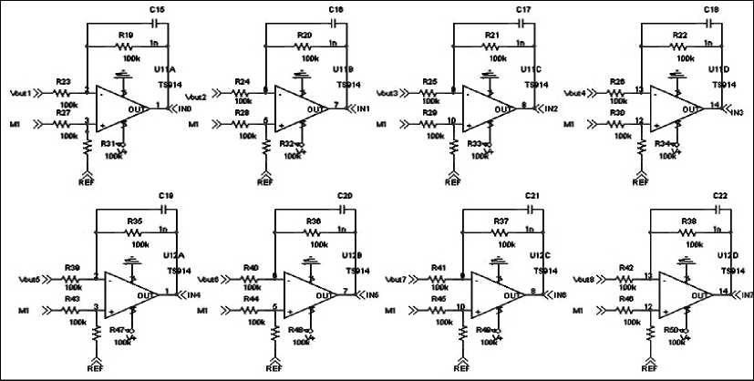
Figure 8. Interference circuit
-
1.5. Modular system
In order to realize modular system, some devices have been introduced. First and more important is operational amplifier (see Fig. 9). Labels M1, M2, M3 in Fig. 9 are joined with corresponding others of different modules, performing parallel configuration. By this way output of two modules was summed and divided by 2, which is the result we wish to obtain in order to realize Grover algorithm for n + 1 q-bits. In fact each module performs three q-bits QSA and by adding a second module we can realize four q-bits QSA. Each module must be unequivocally identified through his address (a selector assign this address on each one), so the control module can send information to a specified module. The control module send bit stream contain- ing address and data to bus. On each module there is a device (74HC85A in Fig. 10) that compares address sent by CPLD with the label of module and, if these are equal, allows it to process data.
Therefore these address indicate which modules must be in third state or which other must communicate through D/A and A/D converters with CPLD (see Fig. 10).
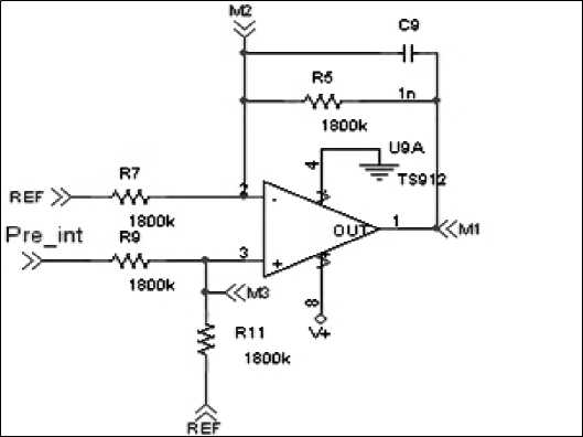
Figure 9. Modular interface, increasing q-bit
As previously reported the control module performs entropy evaluation, vector storing for iterations and output visualization; however its main aim is to manage algorithm iterations.
Control module, that has been realized in digital way (CPLD programmable logic), is able to communicate with Base Modules through addressing system previously described (see in Fig. 11 comparator «74HC85A») and D/A, A/D converters.
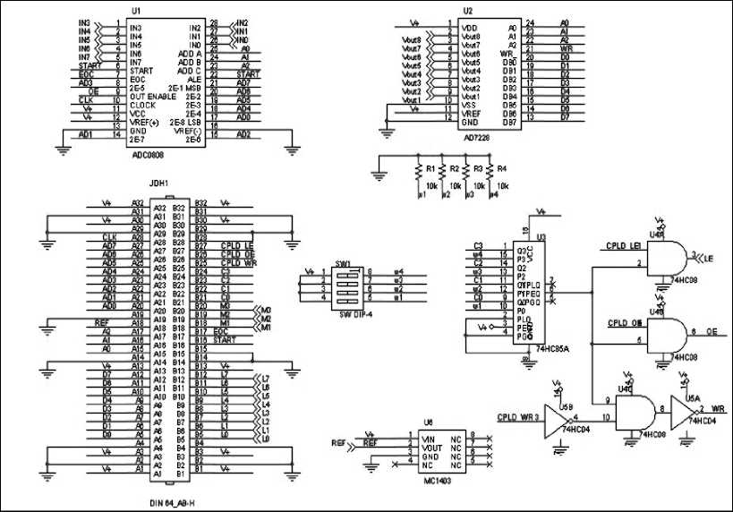
Figure 10. Modular interface, module selection and data conversion
In order to provide the target value (element to be finding) each base module has a latch able to store it (see Fig. 11).
\*
° UW
LE
ID
L1
L3
L4
L5
L6
L7
X 3
X 4
X 7"
X S'
X IT
X 14
CT О
ОС
1D
2D
3D
4D
5D
6D 6
7D§
О О
SDtSQ
2 LC1
5 LC2
6 LC3
9 LC4
12 LC5
15 LCB
16 I.C7
19 i.CS
74Н
Figure 11. Modular interface, latch
General method design of QAGs is developed and is briefly described.
-
1.6. Simulation of a QA-computing on classical computer
Fig. 12 represents a general scheme of Grover's QSA. The Hadamard gates (Step 1) are the basic components for the superposition operation, the operator U (Step 2) performs entanglement operation and D (Step 3) is the diffusion matrix related to the interference operation. Our purpose is to realize some classical circuits (i.e. circuits composed of classical gates AND , NAND , XOR etc.) that simulate the quantum operations of Grover QSA. To this aim all quantum operators must be expressed in terms of functions easily and efficiently described by classical components.
When we try to make the HW components that perform this basic operations according to the classical scheme we encounter two main difficulties.
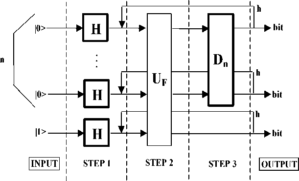
Figure 12. General structure scheme of Grover QSA
Firstly, considering the output of Step 1, we can see that performing a linear number of operations (we have applied the Hadamard matrix n times) we have generated a register state that contains an exponential (2n) number of different terms. In contrast, in classical registers n elementary operations can only prepare one state of the register representing one specific number. Thus, if we simulate a QA with classical HW, add- ing one q-bit implies an exponential increase (2n) in the number of operations to be performed and in the number of gates to be employed.
Secondly , the addition of only one q-bit implies that the matrices U F and Dn ® I dimensions double with respect to the previous configuration and the number of elements (and of products) increases exponentially. Besides most of the computational cost is due to the iterations in the application of UF and D , ® I .
1.6.1. High-level gate design of Grover’s QSA
In this section we present a new HW implementing the functional steps of Grover’s QSA from a high-level gate design point of view. The proposed circuit architectures are modular in the sense that they can be easily generalized by adding similar part according to the desired number of q-bits. By suitable changes in the traditional matrices approach, a 3-q-bits hybrid structure is realized in order to prove the usefulness of gates iterations, which provide a higher probability of finding the exact solution. A minimum-entropy based method in Eq. (2.67) is adopted as a QSA-termination iteration criterion and realized by a digital circuit together with LED display output. The possibility of providing an external clock signal for iteration management allows us to implement a very fast Grover’s QSA (many times faster than the corresponding software realization, and less sensitive to q-bit’s increment.) A modular description of the final circuit is here introduced. According to the high-level scheme introduced in Fig. 12, the proposed circuit can be divided into two main parts.
Part I : ( Analogue ) S tep-by-step calculation of output values . This part is divided into the following subparts:
|
I-a : Superposition ; |
I-c : Pre-Interference (for vector’s approach); |
|
I-b : Entanglement ; |
I-d : Interference |
Part II : ( Digital ) Entropy evaluation, vector storing for iterations and output visualization. This part also provides initial superposition of basis vectors 0 and 1 .
Fig. 13 shows a general structure scheme of the HW realization for the Grover’s QSA-circuits and itself can be considered as a classical prototype of intelligent control quantum system.
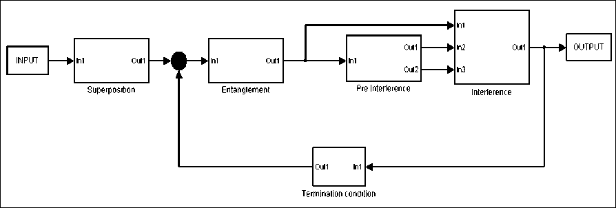
Figure 13. A general SW-scheme of the Grover’s QSA
Example. The most interesting novelty involves the structure of interference: in fact the generic element v (interference output) can be written in function of g (entanglement output) as the following:
П-1Е E g2 j-1 " g- , for i
-
2
"-ЦЕ E g 2 j - g - , for ieven
Referring to Fig. 13, pre-interference operation evaluates a weighted sum of odd (even) output elements of entanglement, while interference itself uses this contribution in order to provide (by means of difference with g ) the respective v . This simple (but powerful) result in Eq. (5) has several consequences.
Remark. Regarding to speed-up of computation, a great improvement has been provided due to the smaller number of products (only one for each element of the output vector) and more precisely 2 n + 1 against
4 n + 1 of the classical approach. Also additions are less than (2 n ( 2 n + 1 ) instead of 4 n + 1). But the most important fact is that all these operation can be easily implemented in HW with few operational amplifiers ( 2 n + 2 ) .
Figs 14 (a), 14 (b) and 14 (c) show the Simulink schematic design and circuit realization of superposition, entanglement and interference operator’s blocks of the Grover’s QAG.
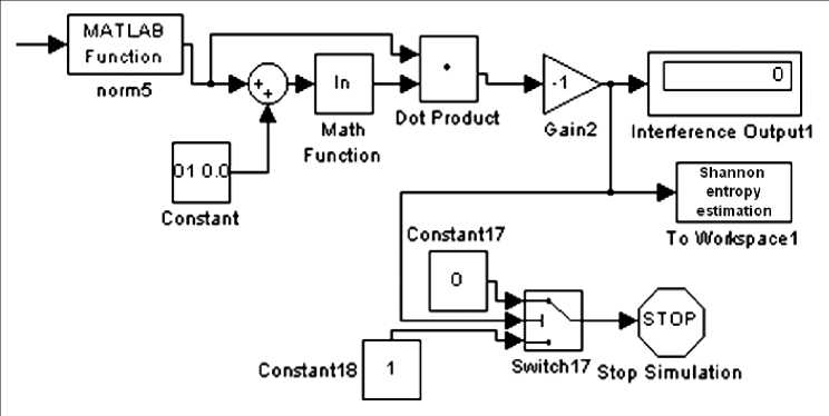
Fig. 14 (b) shows the Shannon entropy scheme estimation for solution of Grover’s QSA termination problem.
Pre-interference sum blocks according to Eq. (5) in Fig. 14 (c) are also reported.
Remark . Fig. 14 shows the main board ( n = 3) for Grover’s QSA that realized the modular structure. Fig. 15 below shows Pre-prototype board implementation of 3-q-bit version of Grover’s QSA. With this preprototype successful experimental simulation results of Grover’s quantum gate Eq. (4) is achieved. Information criteria as minimum Shannon entropy and x 0 = |0^ = 1 as searching element are used. Analysis of these experimental results in detail is developed below.
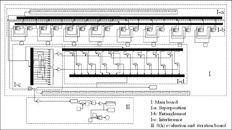
Figure 14 (a). Simulink scheme of 3-q-bits Grover search system
WSTOP
> -1
norm5
Interference Outputl
31 0.C-
Constant
Constantly
To Woikspacel
Suu it ch 17 5tOp Simulation
Constants
Shannon entropy estimation
Math Function
MATLAB Function
Dot Product ^ . . Gain2
Figure 14 (b). Example of the Shannon entropy calculation scheme (Board II of the Fig. 14 (a))
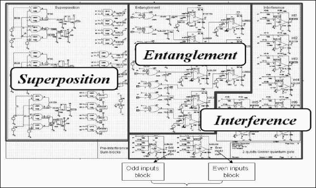
Figure 14 (c). Pre prototype scheme circuit of Grover’s QAG
1.6.2. Experimental testing of Benchmark — Grover’s QAG
According to schematic design solution in Fig. 14 we present in Fig. 15 some photos of HW-implementation and the outputs of the circuit (see Fig. 16) that perform Grover’s algorithm.
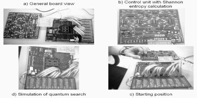
Figure 15. HW-Implementation of Grover’s QSA circuit
We have realized a 3-q-bits accelerator structure for searching in a database constituted by eight elements; this is the reason why eight LED columns are presented in Fig. 16 below that represent the probability of finding each of the database’s elements. We program the entanglement block to find the second element of the database, and repeat four iterations of the algorithm.
Example. Figs 16 (a – d) show the experimental probability evolution of finding each of the database’s elements (from Iteration #1 – to Iteration #4).
At this step (Iteration #2) the probabilities of finding one of the 8 elements of the database are comparable. In the following Fig. 16 (c) the probability of finding the second element of the database begins to increase with respect to the probabilities of finding the others elements. After some other iterations of the algorithm, the difference between the probability of finding the second element and the probabilities to find the others is increased. Finally the probability of extracting the second element of the database is grater than the probabilities of finding any other elements.
Figs 16 (b), 16 (c) and 16 (d) show the evolution of quantum searching using Grover’s QAG. It is a clear demonstration of how we can perform Grover’s algorithm by a classical computer. Similar approach can be used for the realization of quantum fuzzy computing.
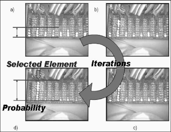
Figure 16. Experimental results of 3-q-bits HW-implementation of Grover’s QSA
Application of Grover’s QAG is a classical efficient simulation process for realization of quantum search computation on classical computer.
Figs 17 and 18 show main 3-q-bits board with modular structure Pre-prototype of Grover’s QSA gate.
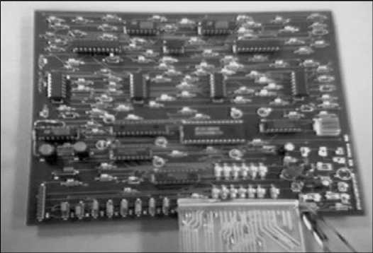
Figure 17. Main 3-q-bits board with modular structure
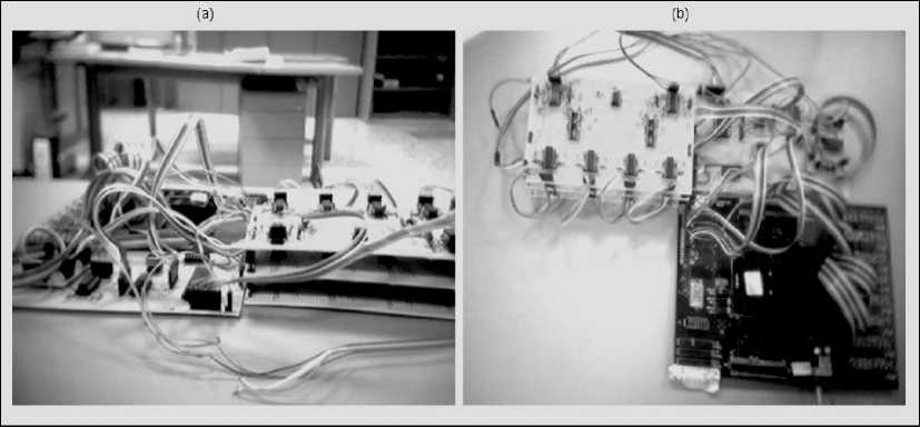
Figure 18. Pre-prototype of Grover’s QSA gate
-
1.7. Software emulator of quantum algorithms
1.7.1. Structure of QA simulation system in MatLab
Fig. 19 shows the structure of a software system for QA simulation.
The software system is divided into two general sections. The first section involves common functions. The second section involves algorithm-specific functions for realizing the concrete algorithms.
Common functions. The common functions include:
-
- Superposition building blocks;
-
- Interference building blocks;
-
- Bra-Ket functions;
-
- Measurement operators;
-
- Entropy calculation operators;
-
- Visualization functions;
-
- State visualization functions;
-
- Operator visualization functions.
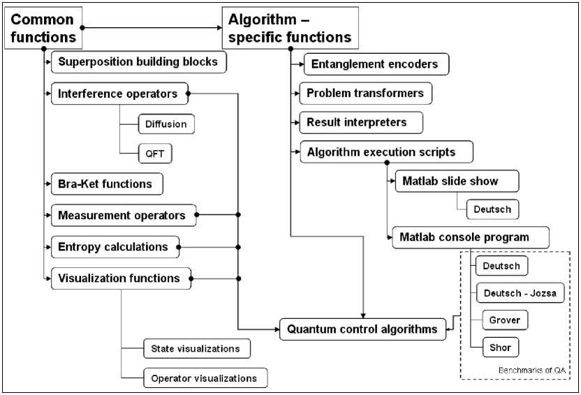
Figure 19. Structure of QA simulation software
Algorithm-specific functions. Algorithmic specific functions include:
- Entanglement encoders;
- Problem transformers;
- Result interpreters;
- Algorithm execution scripts;
- Deutsch algorithm execution script;
- Deutsch Jozsa’s algorithm execution script;
-
- Grover’s algorithm execution script;
-
- Shor’s algorithm execution script;
-
- Quantum control algorithms as scripts.
Visualization functions. Visualization functions are functions that provide the visualization display of the quantum state vector amplitudes and of the structure of the quantum operators.
Algorithmic specific functions. Algorithmic specific functions provide a set of scripts for QA execution in command line and tools for simulation of the QA, including quantum control algorithms. The functions of section 2 prepare the appropriate operators of each algorithm, using as operands the common functions.
Command line simulation of the QAs. The example of the Grover’s algorithm script is presented in Figs 20 – 25.
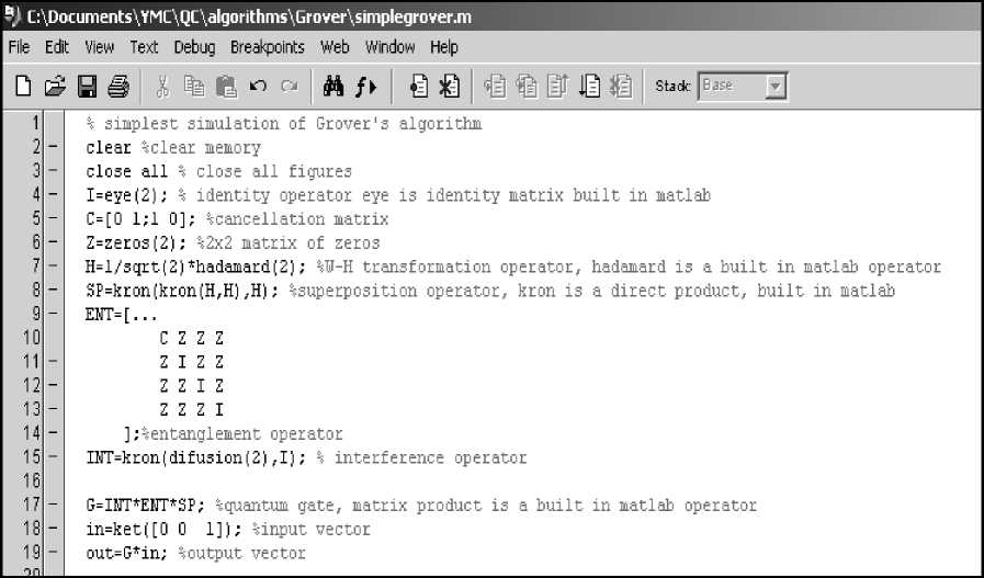
Figure 20. Example of Grover algorithm simulation script (coding of the algorithm)
|
21 22 23 24 25 26 27 28 29 30 31 32 33 34 35 36 37 38 39 40 |
% Plot results of calculations figure(l) subplot(221) plotoperators(SP); title('SP') %plot superposition operator subplot(222) plotoperators(ENT); title('ENT') %plot entanglement operator subplot(223) plotoperators(INT); title('INT') %plot interference operator subplot(224) plotoperators(G); title(1G=INT*ENT*5P1)%plot operator figure(2) subplot(211) plotsuperposition(in); %plot input superposition titled'IN,entropy_{5H} = ' num2str(entropySH(in)) ,1 entropy_{W} = ' numSstrlentropyWIin^in1))]) subplot(212) plotsuperposition(out); %plot output superposition title([1 OUT, entropy_{SH}=' num2str(entropySH(out)) ,' entropy_{W}=' num2str(entropyW(out*out'))]) |
Figure 21. Example of Grover algorithm simulation script (result visualization commands)
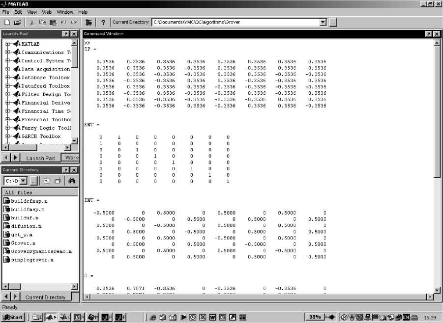
Figure 22. Example of Grover algorithm simulation script (superposition, entanglement and interference operators)
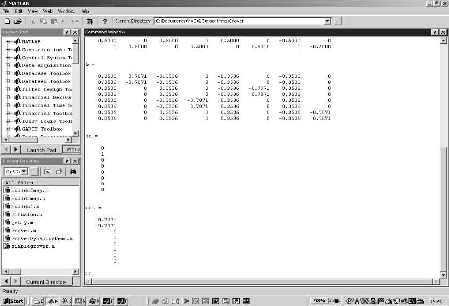
Figure 23. Example of Grover algorithm simulation script (quantum gate G, input vector and result of the quantum gate application)
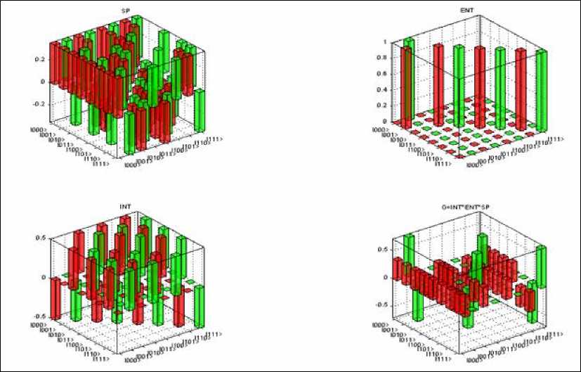
Figure 24. Example of Grover algorithm simulation script (visualization of the quantum operators)
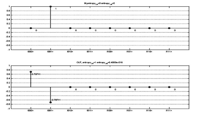
Figure 25. Example of Grover algorithm simulation script (visualization of the input and of the output quantum states)
In Fig. 20, the algorithm-related script is presented. It prepares the superposition (SP), entanglement (ENT) and interference (INT) operators of the Grover’s algorithm with 3 q-bits (including the measurement q-bit). Then it assembles operators into the quantum gate G .
Then the script presented in Fig. 20 creates an input state |in> = |001> and calculates the output state |out> = G |in>. The result of this algorithm in Matlab is an allocation of the operator matrices and of the state vectors in the memory.
Allocated quantum operator matrices are presented in Fig. 22. Allocated input |in> and output |out> state vectors as well as quantum gate G are presented in Fig. 23. In order to see the results, the visualization functions are applied in Fig. 21. Code presented in Fig. 21 displays the operator matrices in Fig. 24 in 3D visualization. In this case the vertical axis corresponds to the amplitudes of the corresponding matrix elements. Indexes of the elements are marked with the ket notation. Input |in> and the output |out> states are demonstrated in Fig. 25. In this case, the vertical axis corresponds to the probability amplitudes of the state vector components. The horizontal axis corresponds to the index of the state vector component, marked using the ket notation.
The title of the Fig. 25 contains the values of the Shannon and of the von Neumann entropies of the corresponding visualized states.
Other known QA can be formulated and executed using similar scripts, and by using the corresponding equations taken from the previous section.
Simulation of the QAs as dynamic systems. In order to simulate behavior of the dynamic systems with quantum effects, it is possible to represent the QA as a dynamic system in the form of a block diagram and then simulate its behavior in time. Fig. 26 is an example of a Simulink diagram of the quantum circuit for calculation of the fidelity of the quantum state and for the calculation of the density matrix |a>
In Fig. 26, input is provided to the ket function. The output of the ket function is provided to the first input of the matrix multiplier and as a second input of the matrix multiplier. Input is also provided to the bra function. The output of the bra function is provided to the second input of the matrix multiplier and as a first input of the matrix multiplier. Output of the multiplier is a density matrix of the input state. Output of the multiplier is the fidelity of the input state.
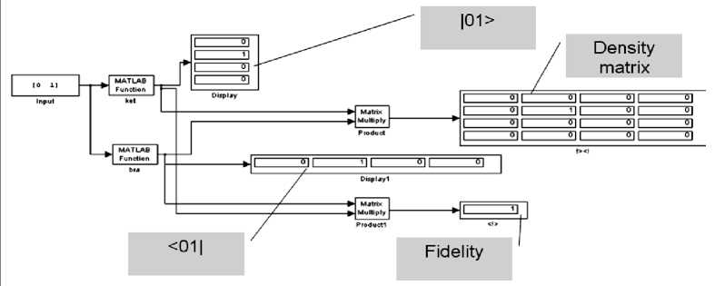
Figure 26. Simulink diagram for the simulation of the arbitrary quantum algorithm
Fig. 27 shows Simulink structure of an arbitrary QA. Such a structure can be used to simulate a number of quantum algorithms in Matlab/Simulink environment.
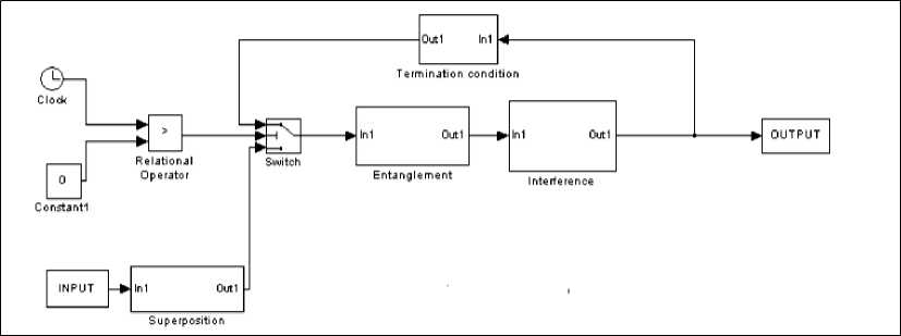
Figure 27. Simulink diagram for the simulation of the arbitrary quantum algorithm
1.7.2. Dedicated QA emulator
Developed in algorithmic representation of QAs is applicable also for design of software emulators of QAs. Key point is the reduction of the multiple matrix operations to vector operations, and following replacement of multiplication operations. This may increase dramatically emulation performance, especially on the algorithms which do not require complex number operations, and when quantum state vector has relatively simple structure (like Grover’s QSA for example).
Developed software can simulate 4 basic quantum algorithms, e.g. Deutsch-Jozsa’s, Shor’s, Simon’s and Grover’s. System uses unified easy to understand interface for all algorithms, with options of 3D visualization of state vector dynamics and of quantum operators.
Startup window of the QA emulator is shown on the Fig. 28. Here one may choose creation of the new QA model or to continue simulation of an existing one.
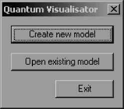
Figure 28. Start-up window of the QA emulator software
If creation of the new model was chosen, then algorithm selection dialog (Fig. 29) will start. Here user may chose QA and its dimensions.
Actually system may operate with up to 50 q-bits and more, but due to visualization problems, it is better to limit number of q-bits to 10 – 11.
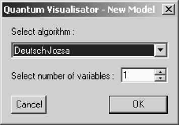
Figure 29. Quantum algorithm creation dialog of the QA emulator software
Once algorithm initial parameters are set, system will draw initial state vector and selected algorithm structure in system’s main window (Fig. 30).
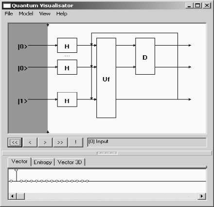
Figure 30. Main window of QA emulator software (3 q-bit Grover QSA)
Main window (Fig. 30) contains all information of the emulated quantum algorithm, and permits basic operations and analysis. Form menu there is an access to involved quantum operators (Fig. 31), and it is possible to modify input functions (see below Fig. 32).
QAs have reversible nature, so by clicking on arrows it is possible to make forward and backward steps of the algorithm, and currently applied algorithm step will be highlighted on the algorithm diagram.
Menu of the emulator consists of four components:
-
1. Item File provides basic operations like project save/load, and new model creation interface access.
-
2. Item Model permits an access to the input function editor (Fig. 32).
-
3. Item View provides an access to operator matrix visualizers, including Superposition, Entanglement and
-
4. From Help menu there is an access to the program documentation.
Interference operators. It is possible to get also 3D preview of algorithm state dynamics (Fig. 34)
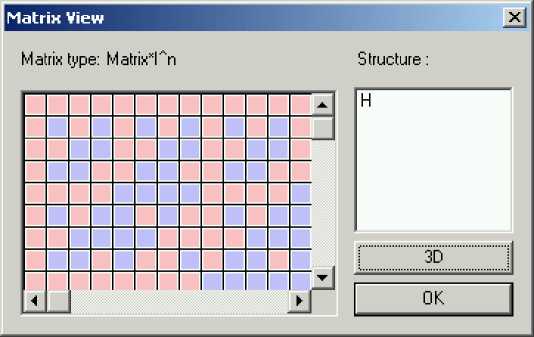
Figure 31. Plain representation of superposition operator
Tabbed interface in the lower part of the window permits an access to Shannon entropy chart and to 3D representation of the state vector dynamics, as well as to usual, plain representation of the QA state. Size of the tabbed area can be modified by dragging divider. Click on the middle point of divider hides tabbed area form the screen.
Buttons in the middle part of the main window permit to make steps of the currently parameterized QA. As it was mentioned above, system can make forward and backward steps.
If enough steps of the algorithm were done, click on the «!» button will extract an answer from the current state vector.
Depending on QA an appropriate result interpretation routine will be called.
Quantum operator visualizer permits to display structure of involved quantum operator matrices in plain (Fig. 31) and in 3D (Fig. 32 (a – c)) representations.
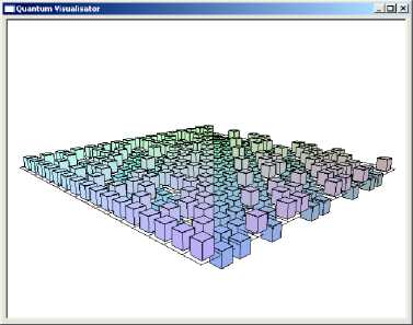
Figure 32 (a). 3D representation of superposition operator of 3-q-bit Grover’s QSA in quantum emulator software
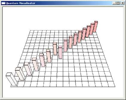
Figure 32 (b). 3D representation of entanglement operator of 3-q-bit Grover’s QSA in quantum emulator software
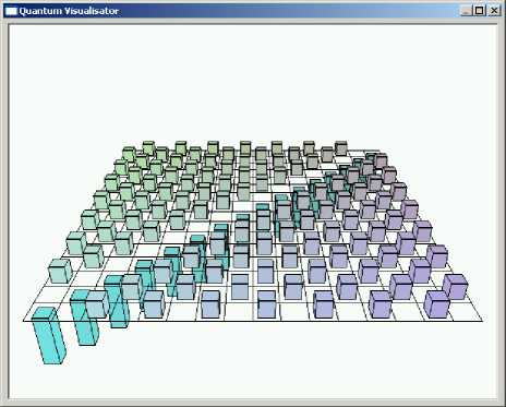
Figure 32 (c). 3D representation of interference operator of 3-q-bit Grover’s QSA in quantum emulator software
If operator consists of tensor product of smaller operators, the possibility to have an access to subblocks of the tensor products is also available. 3D visuzlizer permits zoom and rotation of the charts.
Input function editor permits to automate process of the entanglement operator coding as it was described in previous sections. For Grover’s QSA it is possible to code functions which have more than one positive output (Fig. 33).
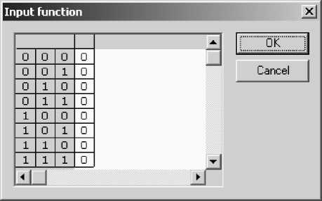
Figure 33. Input function editor of QA emulator (3-Q-bit Grover’s QSA)
Figs 34 – 36 show the results of Grover QSA simulation with entropy criteria termination.
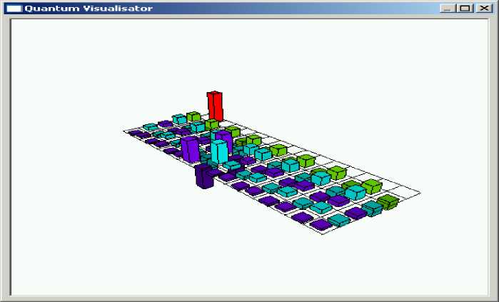
Figure 34. 3D View of 3-q-bit Grover’s QSA state vector after two algorithm iterations
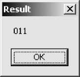
Figure 35. Answer window, case when Grover’s algorithm had performed sufficient number of steps
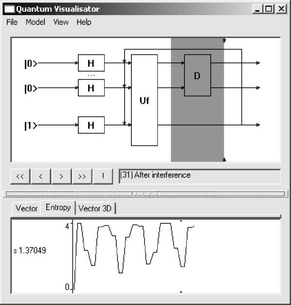
Figure 36. Shannon entropy dynamics after 31 steps of Grover’s QSA
Figs 37 and 38 demonstrate initial (Fig. 37) and final (Fig. 38) states of the developed software emulator with Deutsch-Jozsa’s, Simon’s and Shor’s QAs.
Sample input functions coding and corresponding 3D representation of entanglement operators of Deutsch-Jozsa’s, Simon and of Shor’s algorithms is presented on the Fig. 39.
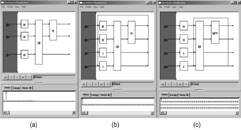
Figure 37. Initial state of QA emulator for simulation of Deutsch-Jozsa’s QA(a), Simon’s QA (b) and Shor’s QA (c)
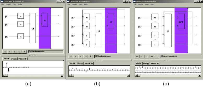
Figure 38. Final state of QA emulator for simulation of Deutsch-Jozsa’s QA(a), Simon’s QA (b) and Shor’s QA (c)
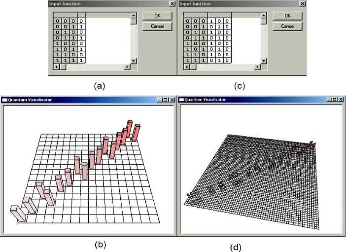
Figure 39. Deutsch-Jozsa’s QA balanced input function (a) and corresponding entanglement operator (b); Simon’s and Shor’s QAs input function (c) and corresponding entanglement operator (d)
Fig. 40 demonstrates Shannon entropy behavior of simulated quantum algorithms after several algorithm iterations. It is clear that its minimum is reached on the states with minimum uncertainty, regardless the simulated algorithm.
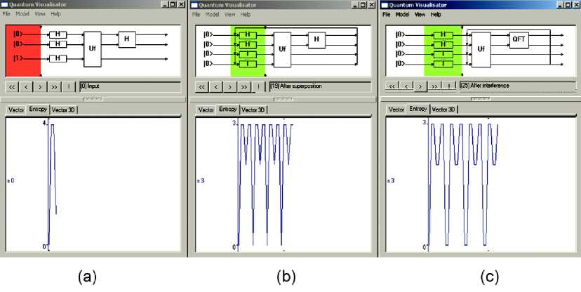
Figure 40. Shannon entropy dynamics. Deutsch-Jozsa’s QA (a), Simon QA(b), Shor QA (c)
Results of QA simulation of simulated QAs are presented on the Fig. 41, after result interpreter.
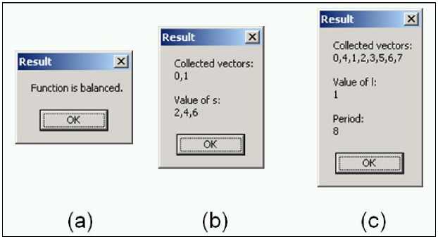
Figure 41. Result interpretation after QA is done. (a) Deutsch-Jozsa’s QA, (b) Simon QA and (c) Shor’s QA
-
1.8. Discussion
Efficient simulation of QAs on classical computer with large number of inputs is difficult problem. For example, to operate only with 50 q-bits state vector directly, it is necessary to have at least 128TB of memory (for the moment largest supercomputer has only 10TB). In present report, for concrete important example as Grover’s QSA, it is demonstrated the possibility to override spatiotemporal complexity, and to perform efficient simulations of QA on classical computers (see Fig. 42).
Design method and hardware implementation of modular system for realization of Grover’s Quantum Search Algorithm are presented. Hardware design of main quantum operators for quantum algorithm gates simulation on classical computer is developed. Hardware implementation for realization of information criteria as minimum Shannon entropy for quantum algorithm termination is demonstrated.
These results are the background for efficient simulation on classical computer the quantum soft computing algorithms, robust fuzzy control based on quantum genetic (evolutionary) algorithms and quantum fuzzy neural networks (that can realized as modified Grover’s QSA), AI-problems as quantum game’s gate simulation approaches and quantum learning, quantum associative memory, quantum optimization, etc.
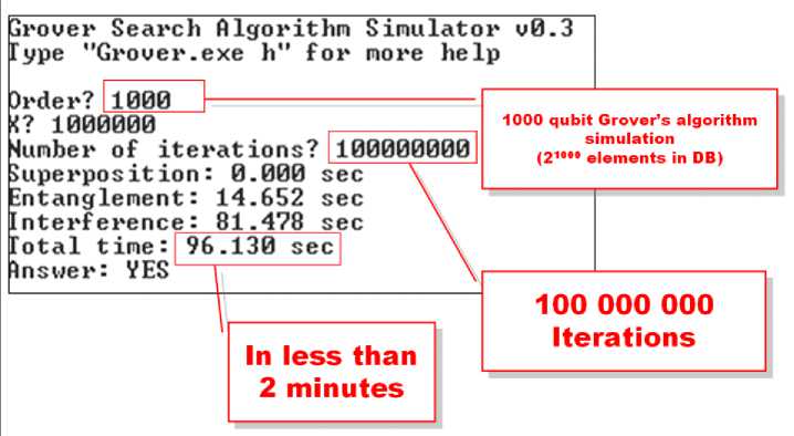
Figure 42. Simulation results of problem oriented Grover QSA according to approach 4 with 1000 q-bits
-
1.9. Comparison of different QA simulation approaches
Fig. 43 shows comparison of the developed approaches of QA simulation.
|
Matrix based approach |
Algorithmic approach |
Problem oriented approach (emulation, superposition is changed with replication, entanglement is realized as element perturbation, interference as a difference equation) |
|||||||||
|
Entire state vector allocation |
Sparse state vector allocation |
||||||||||
|
1 |
2 |
3 |
4 |
||||||||
|
Simulation results (4 qubits, stab |
with minimum of Shannon entr |
opy. x0= |
011) |
||||||||
|
уе^ц^и^ x'1"* । ^"^1 -<^ t^* ^ne'- |
|.™^|U|M^ x^ l x'^-X^ J#”* ^"^ |
||||||||||
|
ОЯЛЖ
1ЛФ1Л1 l-^»«n«n-»4»^UIJ№», .•.--■l |
UUW. unouninnwilner»4i««uej№»- .•.--• Ли . * фи 1 • |
шлю. un№ ieine"cnei-»'фи и- |
шлю. unVW !■-,ЛЖ-ЦИИ»'ЛМ1«1ииЛ>«. .«."И ЛИ . И ФИ 1 . |
||||||||
|
Maximum order reached (number of qubits, simulation on PC with single CPU) |
|||||||||||
|
11+1 (Limited by spatial complexity, matrix approach requires allocation of quantum gate matrix in memory. Gate matrix has a size is 2nx2n) |
19+1 (Limited by temporal complexity, we need 6x10s seconds for one iteration with 20 qubits, and 12x10s seconds for 21 qubits). |
25 qubit (Limited by spatial complexity required for state vector allocation) |
1023+1 without Shannon entropy calculation (Limited by floating point number representation see Figure 3.XX) 64+1 with Shannon entropy calculation (Limited by temporal complexity of calculations) |
||||||||
|
Time required for one iteration with maximum function order (qubit number) on Pill 1GHz (sec) |
|||||||||||
|
103 |
3x10⁵ |
10 |
-0 (q-bit number independent) |
||||||||
|
Remarks |
|||||||||||
|
•Possible introduction of excitation; •Generalized for all OA: •High spatial and temporal complexity. |
•Applicable for hardware realization:
•Additional excitations may double temporal complexity. |
•Impossible introduction of excitations (excitations will cause exponential complexity and algorithm will vanish to 1st approach complexity): •Applicable only to few algorithms: •Simplest hardware realization. |
|||||||||
Figure 43 (a). Results from different approaches for simulation of Grover’s QSA
|
Matrix based approach |
Algorithmic approach |
Problem oriented approach (emulation, superposition is changed with replication, entanglement is realized as element perturbation, interference as a difference equation) |
|
|
Entire state vector allocation |
Sparse state vector allocation |
||
|
1 |
2 |
3 |
4 |
|
Maximum order reached (number of qubits, simulation on PC with single CPU) |
|||
|
11+1 (Limited by spatial complexity, matrix approach requires allocation of quantum gate matrix in memory. Gate matrix has a size is 2nx2n) |
19+1 (Limited by temporal complexity) |
Requires more RSD |
> 1000 (Limited by floating point number representation) |
|
Time required for one iteration with maximum function order (qubit number) on Pill 1GHz (sec) |
|||
|
103 |
10= |
- |
~0 (q-bit number independent) |
|
Remarks |
|||
|
«Possible introduction of excitation; •Generalized for all QA; •High spatial and temporal complexity. |
•Additional excitations may double temporal complexity. |
•Simplest hardware realization. |
|
Figure 43 (b). Results from different approaches for simulation of Deutsch-Jozsa’s QA
In case of Grover’s QSA Fig. 43 (a), shows results from four simulation methods. It is clear that simulation results according with each method are same, but temporal complexity and size of the data base may vary depending on the approach. Direct matrix based approach is more simple, but the q-bit number is limited to 12 q-bits, since operator matrices are allocated in PC memory. The second approach with algorithmic replacement of the quantum gates permits an increase in the degree of the analyzed function (number of q-bits) up to 20 or more. The problem-oriented approach permits quantum gate applications operating directly with the state vector. This permits an exponential decrease in the number of multiplications, and as a result, allows running of Grover’s algorithm on a PC.
|
Matrix based approach |
Algorithmic approach |
Problem oriented approach (emulation, superposition is changed with replication, entanglement is realized as element perturbation, interference as a difference equation) |
|
|
Entire state vector allocation |
Sparse state vector allocation |
||
|
1 |
2 |
3 |
4 |
|
Maximum order reached (number of qubits, simulation on PC with single CPU) |
|||
|
5+1 (Limited by spatial complexity, matrix approach requires allocation of quantum gate matrix in memory. Gate matrix has a size is 2n+m) |
10+1 (Limited by temporal complexity) |
Requires more RSD |
Requires more RSD |
|
Time required for one iteration with maximum function order (qubit number) on Pill 1GHz (sec) |
|||
|
102 |
105 |
- |
- |
|
Remarks |
|||
|
♦Possible introduction of excitation: ♦Generalized for all QA: •High spatial and temporal complexity. |
♦Relatively high function order: •Required specific R&D for each algorithm:
•Additional excitations may double temporal complexity. |
•Applicable only to few algorithms: •Simplest hardware realization. |
|
Figure 43 (c). Results from different approaches for simulation of Simon and Shor’s QA
With this approach, it is possible to allocate in PC memory a state vector containing 25 – 26 q-bits. An extreme version of the Grover’s QSA is an approach when the state vector is allocated as a sparse matrix, taking in consideration that with an absence of decoherence, most of the values of the probability amplitudes are equal, and as a result there is no need to store of all of the state vector, but only the different parts, which is equal to number of the searched elements +1. Thus, excluding memory limitations, one can simulate up to 1024 q-bits or more, with only limitation caused by floating point number representations (with larger number of q-bits, probability amplitudes after superposition approach to machine zero).
In the case of Deutsch-Jozsa’s algorithm simulation, Fig. 43 (b) shows three simulation approaches. In this case, the direct matrix based approach has the same limitations as in Grover’s algorithm, and a PC permits an order up to 11 q-bits. With the algorithmic approach, up to 20 q-bits or more q-bits is possible. The problem-oriented approach with compression gives the same result as in case of Grover’s algorithm.
In case of Simon and Shor’s quantum algorithms, Fig. 43 (c) shows different algorithm structure.
The matrix based approach and algorithmic approach are shown. The matrix based approach permits simulation up to 10 q-bits, and the algorithmic approach permits simulation up to 20 q-bits, or more.
Fig. 44 shows analysis of the quantum algorithms dynamics from the Shannon information entropy viewpoint.
Fig. 44 (a) shows the relation between Shannon information entropy of the state vector of the Grover’s QSA for different parameters of the data base. This analysis permits estimation of the number of algorithm iterations required for database search regarding database size.
The results of Shannon entropy behavior are presented in the Fig. 44 (b) for Deutsch-Jozsa’s algorithm, in Fig. 44 (c) for Simon QA and in Fig. 44 (d) for Shor’s QA.
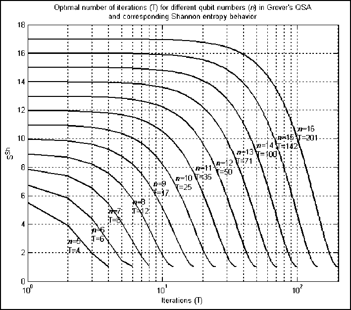
Figure 44 (a). Optimal number of iterations for different q-bit numbers and corresponding Shannon entropy behavior of Grover’s QSA simulation
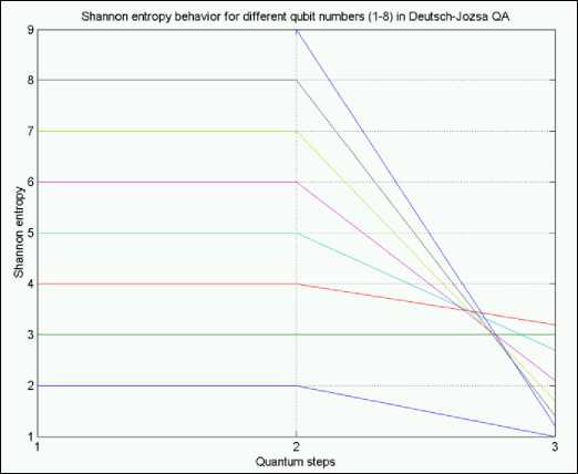
Figure 44 (b). Results of Shannon entropy behavior for different q-bit numbers (1 – 8) in Deutsch-Jozsa’s QA
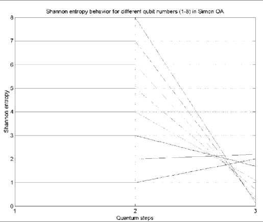
Figure 44 (c). Results of Shannon entropy behavior for different q-bit numbers (1 – 8) in s imon ’ s qa
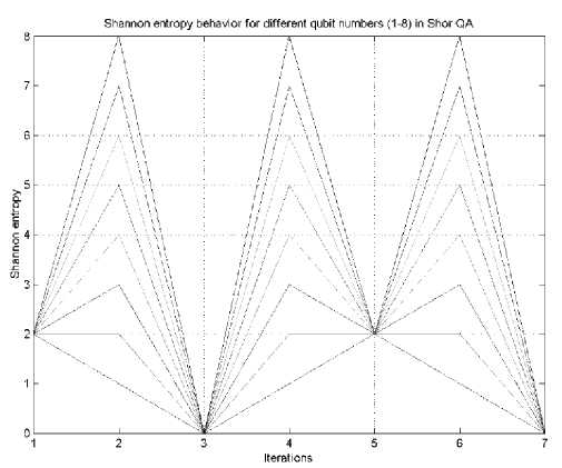
Figure 44 (d). Results of Shannon entropy behavior for different q-bit numbers (1 – 8) in s hor ’ s qa
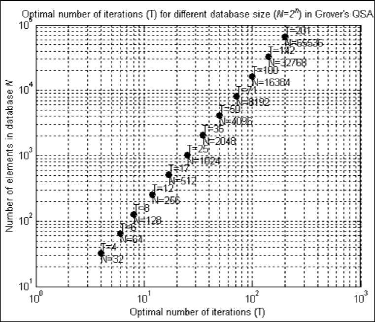
Figure 45. Optimal number of iterations for different database sizes
Fig. 42 shows the screen shot of the Grover’s QSA problem oriented simulator with sparse allocation of the state vector. The result of the simulation for 1000 q-bits is presented.
Fig. 43 summarizes the above approaches to QA simulation. The high level structure of the quantum algorithms can be represented as a combination of different superposition entanglement and interference operators. Then depending on algorithm, one can choose corresponding model and algorithm structure for simulation. Depending on the current problem, one can choose (if available) one of the simulation approaches, and depending on approach one can simulate different orders of quantum systems.
This estimation is shown in Fig. 45.
References General software/hardware approach in acceleration of quantum computing and classically efficient quantum algorithm simulation
- Ulyanov S.V., Litvintseva L.V., Ulyanov I.S. et al. Quantum information and quantum computational intelligence: Classically efficient simulation of fast quantum algorithms (SW&HW implementations). - Note del Polo Ricerca. Milano: Universita degli Studi di Milano Publ. - Vol. 79. - 2004. URL: http://www.qcoptimizer.com.
- Porto D. M., Ulyanov S.V. Hardware implementation of fast quantum searching algorithms and its application in quantum soft computing and intelligent control // World Automation Congress - 5th International Symposium on Soft Computing for Industry, (WAC'2004 - ISSCI). - Seville, Spain. - 2004. - Vol. 17. - Pp. 117-122.
- Ulyanov S.V., Rizzotto G.G. Kurawaki I. et al. Method and hardware architecture for controlling a process or for processing data based on quantum soft computing: Patent US 7 383 235 B1. - 2008.
- Ulyanov S.V., Rizzotto G.G. Takahashi K. et al. Methods and device for performing a quantum algorithm to simulate a genetic algorithm: Patent US 208/0140749 A1. - 2008.
- Ulyanov S.V., Rizzotto G.G. Takahashi K. et all. A method of performing a quantum algorithm for simulating a genetic algorithm. - EP Application. - EP 1 672 569 A1. - 2003.
