Generalized equivalent strength conditions in the calculations of composite bodies

As a rule, the calculation of the strength of an elastic structure is carried out according to the safety factor and is reduced to determining the maximum equivalent stress of the structure (body) [1–3]. For an elastic bodyV0 , the given strength conditions are of the form n1 ≤n0 ≤n2 , where n1 , n2 , are given, the safety factor of the body n0 corresponds to the exact solution of the problem of the theory of elasticity constructed for the bodyV0 . It is believed that the body does not collapse during operation if its safety factor satisfies the specified strength conditions. The determination of the safety factor n0 for a composite body (CB), where is n0= σT /σ0, σT the limit stress σ0 [1], i.e. determination of the maximum equivalent stress [1] CT that meets the exact solution the task of elasticity is difficult. If the stresses in the bodies are determined approximately, then in this case we use the adjusted strength conditions [4], which take into account the error of solutions. In stress-strain analysis (VAT) the finite element method (FEM) is widely used [5; 6].

Finite element (discrete) basic models (BM), which take into account the heterogeneous structure of bodies within the framework of the micro approach [7], have a high dimension. In addition, to analyze the convergence and error of the solution, it is necessary to use the sequence of constructed solutions using the finite element grinding (FE) procedure of BM CB, which leads to a sharp increase in the dimensions of discrete models. For the analysis of CB VAT, the method of multigrid finite elements (MME) [8–14] is effectively used, in which multi-grid finite elements (MNKE) are used and which is a generalization of FEM, since if MNKE is used in FEM, then in this case, in fact, THE CMI is implemented. In the areas of MnKE [8–19], the heterogeneous structure is taken into account and the three-dimensional VAT is described.

It is important to note that MnKE generate discrete models whose dimensions are less than the dimensions of BM CB. For a number of CT (for example, for bodies with a microhedel structure), BMs have such a high dimension that the implementation of FEM using MnKE is also difficult. Existing methods for calculating CT [20–27] are based on hypotheses, have complex formulations and are difficult to implement.

The method of equivalent strength conditions (MESC) is proposed in this paper, to calculate the strength of elastic bodies with an inhomogeneous, microunitive regular structure, which is reduced to the calculation of the strength of elastic isotropic homogeneous bodies using equivalent strength conditions according to feM. Unlike the works [28; 29], the theorem that underlies the MESC is presented in detail here. In numerical implementation, MESC uses adjusted equivalent strength conditions that take into account the error of the solutions. For CB, for which many different loads are specified, generalized equivalent strength conditions are used in the calculations. Implementation of MEPM on the basis of FEM using MnKE requires 10 3 ^ 10 6 times less computer resources than FEM calculation on the basis of grinding BM CT. An example of CB calculation according to MESC shows its high efficiency.

1.    Basic provisions of the method of equivalent strength conditions

MESC is applied to CB that satisfies the following provisions.

Regulation 1. CB consists of multi-module isotropic homogeneous bodies, the connections between which are ideal, i.e. at the general boundaries of isotropic homogeneous bodies, the functions of displacements and stresses are continuous.

Regulation 2. Displacements, deformations and stresses of multimodular isotropic homogeneous bodies correspond to the relations of the linear theory of elasticity [30].

Regulation 3. Approximate solutions of BM CB, built according to FEM, differ from accurate solutions. Such approximate decisions will be considered accurate.

2.    Equivalent strength conditions

Let elastic bodies V1 , V2 have the same characteristic dimensions, shape, fasteners and static loads, but differ in modulations of elasticity. Let for the safety factors n1 , n2 , respectively bodies V1 , V2 , be given strength conditions na ^ n1 ^ nb,                                             (1)

n a ^ n 2 ^ nb,                                            (2)

where n 1 , n 2 >  1; n 1 , n 2 , n 1 , n 2 are given; the reserve coefficient n ( n₂ ) corresponds to the exact solution of the problem of the theory of elasticity, built for the body V (body V ).

For bodies V , V , enter the following definition.

Definition. If from the fulfillment of conditions (2) for the coefficient n follows the fulfillment of conditions (1) for the coefficient n and vice versa, if from the fulfillment of conditions (1) for the coefficient n follows the fulfillment of conditions (2) for the coefficient n , then the conditions of strength (1), (2) will be called equivalent conditions of strength co-responsible for bodies V , V .

3.    Basic theorem of the method of equivalent strength conditions

Without losing the generality of judgments, we consider bodies with a fibrous structure, which are widely used in practice and in which the maximum equivalent stresses arise in the fibers. The MESC is based on the following theorem.

Theorem 1. Let the load and strength conditions of the form F be set for the safety factor n of the elastic CT (fibrous structure)

n 1 <  n 0 <  n 2 ,                                             (3)

where the values n , n ₂ are given, n >  1, n₀ = °_r / o₀ , °_T , is the limit stress of CT (the yield strength of the fiber), o₀ is the maximum equivalent stress of CB V_o , the stress °₀ corresponds to the exact solution of the problem of the theory of elasticity, built for loading F CB V , the body fibers V have the same modulus of elasticity.

Let the homogeneous isotropic body V b and CB V have the same shape, characteristic dimensions, fastenings and loading F . Let the elastic modules of the body V b and the CB fibers are the same. Then there exists such a number p > 0 (equivalence coefficient) that if the safety factor of the body Vb satisfies the adjusted equivalent conditions of strength pn1

1 — 5_a

< ⁿ b <

pn ₂

1 + 5_a ,

then the safety factor n ₀ CB V ₀ meets the specified conditions of strength (3), where , n_b = ° _T / о _b is a _b the maximum equivalent stress of the body V^b , corresponding to the numbered solution constructed for loading the body with an error 5 _b , | 5 _b | < 5_a , where 5_a is the upper estimate of the error 5 _b , satisfying the condition

5a< Сa= (n2 - n1)/(n2 + n1)

Proof.

Safety factor n0 , n0 , respectively bodies V0 , Vb are found by formulas n0 = °T I °0, nb = ° T 1 ° b, where n0 is the maximum equivalent stress of the body Vb corresponding to the exact solution of the problem of the theory of elasticity constructed for loading F the bodyV b .

Let the coefficient n satisfy the conditions (3). Using (6) in (3), we have n1 < — < n2 .(8)

^c 0

There is such a number p >  0 (equivalence coefficient) that

p(9)

^c b

Given (9) in (8), we get

Pn1 <^0 < Pn2.

• ^c b

Using (7) in (10), we have

РП1 < nb < РП2.

Let the body's V^b safe factor n ⁰ satisfies the conditions of strength (11).

РcT

Then, substituting (7) in (11) with (9), we have pn < ——— <  pn . From where, taking into account ^c 0

(6), the strength conditions for the CB safety factor V (3) follows. Let’s consider the limit cases.

Let n 0 = pn . Using the relations (7), (9) in the last equality, we obtain p — = pn . From where , ^c 0

taking into account (6) n ⁰ = pn follows. Similarly, we show that if n ₀ = n ₂, the n ⁰ = pip then .

CT

Let n ₀ = n 1 . Using (6), (9) in the last equality, we get —T = pn . From where, taking into account ^c b

• (7)    follows n ⁰ = pn . Similarly, we show that if n ₀ = n ₂ , then n ⁰ = pip . So it is shown that (11) are equivalent strength conditions for CB V ₀ (see definition of paragraph 2). Let the maximum equivalent stress c _b e be found for the body V^b such that

15ь |<5a< C.   (n2 -n1)/(n1 + n2),(12)

where 5 _b is the relative error for c _b , i.e.

.

5 b = (cb-c 0)/cb\

From (13) follows cb = (1 + 56) c0. From here, considering (7) and that nb =cT / cb , we get nb = (1 + 5 b) nb.(14)

Note , that in (12) C _a< 1. Let 5 ₀ = | 5 _b |. Then due to (12)

0<50 = 15b | <5a< 1.(15)

Taking in (14) 8b = -80,5j =50 sequentially , enter the coefficient nr = (1 -5o)nb, n2= (1 + 5o)nb.(16)

Then due to (14), (16) we get nb = n[ or nb = n 2(17)

Let’s enter the coefficients nd ,nd according to the formulas nd = (1 -5e)nb,  n2d = (1 + 8a )nb .(18)

Because of 0 <  8_a <  1, n_b >  0, it follows from (18)

nd < n2d .(19)

Adjusted equivalent strength conditions are of the form (4) or pn1(1 + 8o ) < nb (1 -Sa ) < pn 2(1 -8O ),(20)

where n_b = a_T / a_b , o_r , is the limit voltage of CB (the yield strength of the fiber).

Let n the conditions of strength (20) be fulfilled, i.e. let pn < (1 -8o ) nb and(1 + 8o )nb < pn2 Then it follows that for coefficients nd , nd , taking into account (18), (19) inequalities are fulfilled pn1 < nd < n2 < pn2.

Comparing (16), (18) taking into accounts (15), the inequality n d <  n[ , n 2 <  n d follow.

Hence, given, that according to (16) n2 < n2 , we get drrd n1 < n1 < n2 < n2 .(22)

Then by virtue of (21), (22) inequalities are fulfilled pn1 < nr < n2 < pn2 .(23)

From the implementation (23) taking into account (17) follows the fulfillment of the conditions of strength (11) for the reserve factor n ⁰ , therefore, the fulfillment of the specified conditions of strength (3). The constraints on the parameter 8_O are found from the condition of existence of strength conditions (4), i.e. let pn 1 (1 + 8_O ) <  pn ₂(1 -8_O ) .Where it comes from

• ⁸o< Co=⁽n2 ^-n1^)/(n1 ⁺n2).                                ⁽²⁴⁾

4.    Implementation of the method of equivalent strength conditions

Since n ₂ >  n 1 >  1, then from (24) it follows 0 <  C _O<  1 . If 8_O = C _O , then from (4) it follows n_b = p ( n 1 + n 2 )/2 that it is difficult to perform in practice. Therefore, you should specify such 8_O that 8_O<  C _O .

In this case, the conditions (11) for the bodyVb safety factorn0 can be met using adjusted equivalent strength conditions (4) and numerical solutions that generate such errors 8b for body Vb stresses that| 8b | < 8O . It has been shown that the fulfillment of conditions (11) follows the fulfillment of strength conditions (3). The theorem is proven.

According to theorem 1, the implementation of the MESC is reduced to the determination of the coefficient p and the safety factor n_b of the body V ^b , i.e. to the determination of the maximum equivalent stress a _b of the body V^b with an error | 8 _b | < 8_O , n_b = a _T / a _b .

Without losing the commonality of judgments, for simplicity of presentation, the procedure for implementing the MESC will be considered on the example of a body V with an inhomogeneous regular structure of sizes H x H x H , where H = 6 Nh , N is the whole, N >>  1, h little. CB V_o , located in the Cartesian coordinate system Oxyz , with y = 0 rigidly fixed, i.e. at y = 0: u , v , w = 0 . The regular cell G CB V , having the shape of a cube with a side 6 h , is located in the local Cartesian coordinate system Oxyz , i , j , k = 1,...,7 (Fig. 1), the fibers are directed along the axis Oy by cross-section h x h , the fiber sections are painted over. So, the body V is reinforced with pa-rally axes Oy of continuous fibers. Strength conditions (3) are set for CB V . BM R CB V , consisting of finite elements (CE) V ^h of the 1st order of the shape of the cube with a side h (in which the three-dimensional VAT is realized), takes into account the heterogeneous structure of the body V and generates a uniform grid with a step h . We think that 3 MESC for CB V is performed.

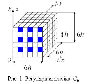
Fig. 1. Regular cell G ₀

Note that the implementation of the MESC is reduced to the determination of the equivalence coefficient p , the body V ^b reserve coefficient n_b and the construction of adjusted equivalent strength conditions (4).

Finding the equivalence coefficient p

According to the MESC, we will introduce an isotropic homogeneous body V ^b and CB as R ⁰ are follows that the bodies V ^b , R ⁰ and V ₀ have the same shape, characteristic dimensions, given fastenings and loads, but differ in modulations of elasticity. The moduluses of elasticity of the body V ^b are equal to the modules of elasticity of the CB V ₀ fiber. For the body V ^b (for CB R ⁰ ) we define discrete models уП (models R ^ ) that form sequences {V } N = 1 , { R 0 } ^N = 1 . The model V Nb is BM body V^b . The model уП (model R_n ⁰ ) consists of CE V ^{( n )} 1st order of cube-shaped FE with a side h_n in which a threedimensional stress state is realized and that generates a uniform grid with a dimension n ( ⁿ ) x n 2 ⁿ ) x n 3 ⁿ ) , step h_n , where

n ( ⁿ ) = 6 n + 1, n 2 ⁿ ) = 6 n + 1, n 3 ⁿ ) = 6 n + 1, n = 1,..., N .                       (25)

According to (25), the model Vb (modelR0 ) consists of a finite number of isotropic homogeneous bodies Gb s (CT G0) of the same shape and size , with dimensions 6hn x 6hn x 6hn , where hn = H /(6n) = pnh ,                                    (26)

where H = 6 Nh , в _n = N / n , n = 1, N at n <  N : в _n >  1, h n >  h , when n ^ N we have h n ^ h , h_N = h .

CB G 0 has the same number of grid nodes (343 nodes), the number of fibers (cross-section h_n x h_n ) and the same mutual arrangement as a regular cell G (Fig. 1). Fibers and matrix CB G ⁰ and G have the same modules of elasticity n = 1, N , (Fig. 2), where h_n >  h at n <  N , i , j , k = 1,...,7.

C B G ⁰ , G , (their heterogeneous structures) geometrically differ only in scale. For the convenience of reasoning, formally for CT G ⁰ , G , let’s write down the ratio

G n = в n G 0 ,                                       (27)

where в _n is the scale coefficient, в _n = N / n , n = 1, N , at n ^ N : в _n ^ 1, в _N = 1, G N = G 0 .

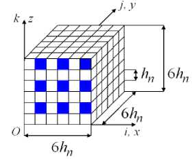
Рис. 2. КТ G ⁰ (регулярная ячейка модели R ⁰ )

Fig. 2. CB G ⁰ (regular cell body R ⁰ )

Note that since in the regular cell G ₀ the heterogeneous structure is taken into account, then due to (27) and in CB G ° ( n = 1, N )the heterogeneous structure using the CE Vj ^{( n} ) of the 1st order of the shape of the cube with a side h_n is also taken into account, i.e. the model R ⁰ takes into account the heterogeneous structure. Note that CB G ⁰ , in fact, is a regular cell of the model. So, the models V^b , R ⁰ have the same shape, dimension, the same characteristic dimensions, uniform grids with a step h_n , fastening and loading, like CB V ₀ , i.e. models V^b , R ⁰ , differ from each other only in modulations of elasticity. Note the following advantages of the models V^b , R ⁰ .

• 1.    Dimensions of models V b , R n with n <  N the force of (25), (26) less than the dimension of BMR₀ .

• 2.    When building models { R ° } N = 1 , BM R₀ grinding is not used.

To reduce the dimensions of the models V^b , R ⁰ , multi-grid FE are used.

Due to (26), (27) at n = N ( h_N = h , β _N = 1 i.e. G ⁰ = G ) models V^b , R ⁰ , and BM R ₀ CB V ₀ have the same dimension, and models R ⁰ and R in force (27) coincide, i.e. R ⁰ = R . Since, according to (27), at n → N we have G ⁰ → G , then we get

Rn0→RN0=R0 at n→ N.(28)

Since the models R ⁰ , V^b , have the same dimension as the BMR , for which the positions 3 MESC are executed, then we consider that the maximum equivalent stress σ ⁰ (stress σ ^b ) of the model R ⁰ (model V^b ) differs little from the exact σ ( σ ⁰). Therefore, we believe that

σ0 = σN , σb= σN,(29)

where σ ⁰ is the maximum equivalent stress of the body V ^b corresponds to the exact solution of the three-dimensional problem of the theory of elasticity constructed for the body V^b .

The equivalence coefficient p is found by the formula (9), i.e. p = σ / σ ⁰ or including (29)

p = σ0N/ σbN.(30)

The approximate value of the equivalence coefficient p is found by the formula pn =σ0n/σbn,(31)

where σ ⁰ ( σ ^b ) is the maximum equivalent stress of the model R ⁰ (model V^b ).

Due to (26) at V^b → V^b , n → N should follow . Hence, given (28), we have

σ0n→σ0N, σbn→ σbN at n→N.(32)

Taking into account (32), (29), (30) in (31), we get pn → p at n→ N.(33)

Let it be δn =| pn - pn-1 | /pn few where n =2,3,.... Then we accept p= pn .(34)

Calculations show uniform (monotonous) convergence of stress σ ⁰ , σ ^b , and parameter p_n respectively to stress σ ⁰ , σ ^b , and parameter p .

Construction of adjusted equivalent strength conditions

Substituting the found equivalence coefficient p and given values of δ _α , n ₁ , n ₂ in (4), we determine the adjusted equivalent strength conditions for CB V ₀ .

Finding a safety factor n_b for a homogeneous isotropic body V ^b

Let it be δ _n ^σ = | σ ^b _n - σ ^b _{n - 1} | / σ ^b _n few and| δ^σ _n | ≤ δ_α , where δ_α< C _α , n = 2,3,.... Then we assume

σ b =σ ^b n .                                        (35)

Using (35) in the formula n = σ /σ , we determine the safety factor n for the body Vb nb = σT / σbn .

Checking the specified strength conditions

Let the safety factor of the isotropic homogeneous body V ^b found by the formula (36), i.e., corresponding to the numerical solution of the elasticity problem, satisfies the adjusted equivalent strength conditions (4) constructed for CB V . Then, according to theorem 1 (see paragraph 3), the safety factor n of CB V , corresponding to the exact solution of the elasticity problem satisfies the specified conditions of strength (3).

The procedure for constructing generalized equivalent strength conditions for CB V , for which many different loads are specified, without losing the commonality of judgments, will be considered with the CB V example. Let on the surface S of the CB the loading of the form q , q , q acts, where q , q , q are the surface loads acting respectively in the direction of the coordinate axes Ox , Oy , Oz ; q_x , q_y , q_z ∈ Q_xyz , Q_xyz is a set of different loads given for CB V ₀,

Q_xyz = { q_x , q_y , q_z : q_x , q_y , q_z - гладкие функции, заданные на S } (37) smooth functions given on S. ВСТАВИТЬ ТЕКСТ

To find the (upper, lower) boundaries for the set P of equivalence coefficients corresponding to the load set (37), we calculate for a number of characteristic loads of CBV0 : qx= qx(n), q= q(n), q= q(n) (q(n), q(n), q(n) smooth functions), n= 1, N, N - given. Enter the coefficients p1 = min(p(n)) , p2 = max(p(n)) , n= 1,N0 , т. е. ∀p ∈P : p1≤p ≤p2.(38)

Let the condition for CTV0 be met p2C1 ≤ p1C2 ,(39)

where is C ₁ = n ₁/ (1 - δ_α ) , C ₂ = n ₂/(1 + δ_α ) .

For the equivalence coefficient pq ∈[ p1, p2]  , which is found by FEM for body load ing qx , qy , qz ∈ Qxyz , the strength conditions (4) take the form pqC1≤nb ≤pqC2,(40)

where n_b is the safety factor of the isotropic homogeneous body V ^b .

According to (38) we have pqC1 ≤ p2C1 , p1C2 ≤ pqC2 . Using these inequalities and (39), we get pqC1 ≤ p2C1 ≤ p1C2 ≤ pqC2 . Let the loading of the bodyqx, qy, qz ∈ Qxyz be such that pqC1 ≤ p2C1 ≤nb ≤ p1C2 ≤ pqC2 ,(41)

i.e. the following conditions of strength are met for the body V b safety factor nb p2C1≤nb≤p1C2.(42)

Let the coefficient nb   for the bodyV b satisfies the conditions of strength (42) for load ing qx , qy , qz ∈ Qxyz . Then the conditions (41) are met for the coefficient nb , i.e. the conditions of strength (40). According to theorem 1 (see paragraph 3), from the fulfillment of the conditions of strength (41) follows the fulfillment of the specified strength conditions (3) for loading qx, qy, qz e Qxyz CB Vo . Note that according to the MESC, the body Vb and the CB Vo have the same loads (see paragraph 4). Thus, it is shown that from the fulfillment of the conditions of strength (42) for a body having a load, the fulfillment of the strength conditions (3) follows for loading qx, qy, qz e Qxyz CT Vo . Conditions (42) will be called generalized equivalent conditions of strength. In fact, the following statement is proved above.

Theorem 2. Let for the set Q of different loads given for CB V , according to the MESC, generalized equivalent strength conditions (42) are constructed. Let for the reserve factor n of an isotropic homogeneous body V b having a load F e Q , the strength conditions (42) are met. Then the specified strength conditions (3) for loading F CB V are met.

6.    Results of numerical experiments

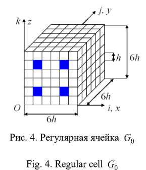
Consider the model problem of calculating the strength of a cantilever composite beam V , the dimensions H x L x H , where H = 96 h , L = 1152 h , h is given (Fig. 3). The regular cell G _o of CB V _o has the shape of a cube with a side 6 h , the fibers h x h are parallel to the axis Oy (Fig. 4), the fiber sections in the plane Oxz are painted over. So, the body V is reinforced with parallel axes Oy with continuous fibers, the distance between the fibers is 2 h . When y = 0 CT V _o is rigidly fixed and at z = H has a load of the form q_x , q_z , where q_x ( q_z ) is the force acting on the beam in the direction of the axis Ox (axis Oz ).

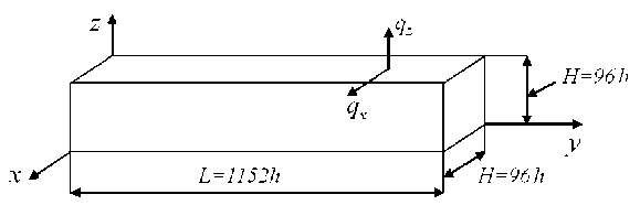
Рис. 3. Размеры тела V ₀ (тела V ^b , моделей V^b , R ⁰ )

Fig. 3. Dimensions of the body V ₀ (body V ^b , models V^b , R ⁰ )

The basic discrete model R ₀ of CB V ₀ , consisting of single-grid finite elements (1 cCE) V^h of the 1st order of the cube shape with a side h [5; 6] (in which the three-dimensional VAT is implemented [30]), takes into account the heterogeneous structure of the body V ₀ and generates an equal-dimensional (basic) grid with dimension 97 x 1153 x 97 step h . Fig. 4 shows the base grid of the regular cell G ₀ . Since the BM R ₀ has 32517504 (over 32 million) unknown FEMs and since h / H <<  1 ( h / H = h / (96 h ) = 0,0104), we will assume that the maximum equivalent voltage of the BM R ₀ differs little from the exact solution, i.e. put. 3 MESC for CB V ₀ is performed (see paragraph 1).

For the CB V safety factor n , the strength conditions of the type are set

.                                          1,3 <  n 0 < 3,5.                                          43)

Initial data for CB V0: h = 0,2083; aT = 5; vc =vv = 0,3 Ec = 1, Ev = 10 , whereEc, Ev (vc, vv )are the Jung modules (Poisson coefficients) respectively of the binder material and fiber, on the surface S = {0,5L < y < L, z = H} of the CB Vo there is a uniform loading qz = qx = 0,000285, aT is the yield strength of the fiber.

According to the MESC, we will introduce an isotropic homogeneous body Vb and CBR0 such that the bodies V b , R0 and V have the same shape, characteristic dimensions, given fastenings and loads, but differ in modulations of elasticity. Body V b elasticity modules are equal to fiber elasticity moduluses CBV . For the body Vb (for CBR0 ) define discrete models Vb (modelsR0 ) that form sequences {Vb}16 , {R0}16 . The modelVb (modelR0 ) consists of a 1st order cube shaped 1cCEV(n) with a side hn in which the three-dimensional VAT is realized and which generate a uniform grid with a dimension n(n) x n2n) x n3n) step hn , where n1(n) = 6 n +1, n 2n) = 12 x 6 n +1, n 3n) = 6 n +1, n = 1,2,3,....                    (44)

The steps h(n), h(n), h(n) of the grids of the model Vb (modelR0 ) respectively along the axis Ox , Oy , Oz , are equal to h(n) = H/(6 n), h(n) = L/(72 n), h(n) = H/(6 n) . Since L = 12 H, then hn = h(nn) = h(n) = h(n) . From here, given that H = 96h , we get hn = Pnh ,                                             (45)

where в _n = 16/ n , n = 1,2,3,..., at , n <  15 в _n >  1, h_n >  h .

According to (44), the model V_n^b (model R_n ⁰ ) (Fig. 3) consists of a finite number of isotropic homogeneous bodies G b (CB G 0 ) of the same shape and size 6 h_n x 6 h_n x 6 h_n (Fig. 5).

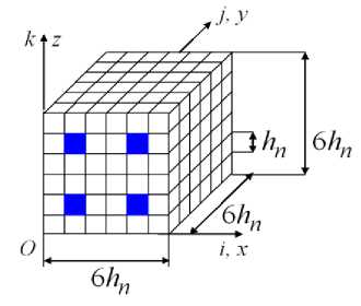
Рис. 5. Регулярная ячейка G ⁰

Fig. 5. Regular cell G ⁰

CB G 0 has the same number of fibers (cross-section h_n x h_n ) and their same mutual arrangement as a regular cell G (Fig. 4), fibers and binder material CB G ⁰ and G have the same modules of elasticity n = 1,16 . So, CB G 0 , G _o, (their heterogeneous structures) geometrically differ only in scale. Then, for the convenience of reasoning, taking into account (45), for CB G ⁰ , G we formally write down the ratio

G n = P _nG 0 ,                                        (46)

where P_n is the scale coefficient, with n ^ 16 , we have P„ ^ 1 , P₁₆ = 1 , i.e. G 106 = G о .

Note that since the regular cell G takes into account the heterogeneous structure, then due to (46) and in CB G 0 ( n = 1,2,3,...) the heterogeneous structure is also taken into account with the help of 1cCE V ^{( n )} of the 1st order of the shape of the cube with a side h_n , i.e. the model R ⁰ takes into account the heterogeneous structure. Note that CB G ⁰ is essentially a regular cell of the model R °, n = 1,2,3,... . So, the models V^ , R ° have the same shape and dimension, the same characteristic dimensions, uniform grids with step h_n , fastenings and loads like CB V ₀ .

In the calculations we use two-grid FE (2sKE). When constructing a 2sCE V _d ⁽²⁾ with dimensions 6 h x 6 h x 6 h [15-19], we use two nested grids: a small uniform grid h d with dimension 7 x 7 x 7 step h and a large grid H d of dimension 2 x 3 x 2 , H d c h d . Along the axes Oy , Oz the grid H _d has a step 6 h , along the axis - a step. 3 h On Fig. 6 grid H _d nodes marked with dot 12 knots. The grid h _d is generated by the basic partition of R _d 2cKE, which consists of 1cCE V^h of the 1st order of the cube shape with a side h (in which the three-dimensional VAT, j = 1,..., M is realized, M is the total number of 1sKE V^h , M = 216 ) and takes into account the heterogeneous structure of the 2sKE V_d² 2 .

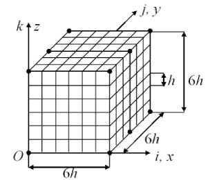
Рис. 6. Мелкая и крупная сетки 2сКЭ V ⁽²⁾

Fig. 6. Small and large grids 2gFE V ⁽²⁾

On the partition R we build a superelement V using the condensation method [5]. The total potential energy П of the superelement V is represented in the form of

П_S =   q ^T _S [ K_S ] q _S - q ^T _S F _S ,

where T is transposion; [ K ] is the matrix of stiffness (dimension 654 × 654 ); F , q are the vectors of nodal forces and displacements (dimensions 654 ) of the superelemen V t. The basic func-tion N_ijk ( x , y , z ) for the node i , j , k of a large grid H_d using Lagrange polynomials is written in the form N_ijk = L_i ( x ) L_j ( y ) L_k ( z ), where

23                                2

L i ( x ) = ∏ ^{x - x α} , L j ( y ) = ∏   ^{y - y α} , L k ( z ) = ∏   ^{z - z α} ,

α=1,α≠i xi - xα           α=1,α≠j yj - yα           α=1,α≠k zk - zα where xi,yj,zk are the coordinates of the grid Hd node i,j,k in the coordinate system Oxyz ; ijk is an integer coordinate system introduced for grid nodes Hd , i,k= 1,2 ; j = 1,2,3 (see Figure 6).

denote: Ne =Nijk, ue =uijk,  ve = vijk , we = wijk , where uijk,  vijk, wijk are the values of the movements u, v, w in the gridHd , i,k= 1,2, j = 1,2,3 , e = 1,...,12 nodei,j,k , Then the approximation functions of displacements u(2) , v(2) , w(2) , 2sKEV (2) represent

12                       1212

u(2)=∑Neue, v(2)=∑Neve,w(2)=∑Newe.(48)

e=1                      e=1

Denote: q _d – vector of nodal displacements of a large grid H_d (dimension 36), i.e. vector of nodal unknown 2sKE V ⁽²⁾ . Using (48), the vector q _S of nodal displacements of the superelement V_S is expressed through the vecto q _d r , i.e.

qS=[ASd] qd,(49)

where [ A^d ] is the rectangular matrix (dimensions 654 × 36 ).

Substituting (49) in (47) we get П S = П _S ( q d ). From the execution д П _S / d q d = 0 we obtain the equality [ K_d ] q _d = F _d , where [ K_d ] = [ A_S^d ] ^T [ K_S ][ A_S^d ] , where[ K_d ], F _d , is the matrix of stiffness (dimension 36 × 36 ) and the vector of nodal forces (dimension 36) 2cCE V ⁽²⁾ .

The solution built for the 2cCE V ⁽²⁾ grid H is projected using the formula (49) on the grid of the superelement V , then using the ratios of the condensation method - on a fine grid h of 2cKE V ⁽²⁾ which allows you to find voltages in 1sKE V^h basic partitioning R 2cKE V ⁽²⁾ .

On the model V^b ( R ⁰ ) we build a two-grid discrete model, which consists of a 2cCE type V ⁽²⁾ of size 6 h_n x 6 h_n x 6 h_n , where h_n = 16 h / n , n = 1, 11 and which we denote V 0 ( R_n ). Note that the models V 0 , R , have the same dimension. For models V ⁰ , R , we find (according to the 4th theory of strength [1]) respectively the maximum equivalent stresses c b , C 0 , n = 3,5,...,11. . The results of the calculations are presented in Table. 1, where

5 p (%) = 100% x | p n - p n — 2 |/ p n , (50) where n = 5,7, 9, 11; p_n = c 0 / c b ; N O , b oo are the dimension and width of the tape SU FEM model V 0 , n = 3,5,...11.

The analysis of the results of the calculations shows a uniform monotonous convergence of the stress c b , c 0 , parameter p_n and error 5 p . Let’s consider the calculation of CB V_o on the basis of BM. Note that in CB calculations, as a rule , three (or more) discrete models are used to analyze the convergence and error of numerical solutions. In this case, we use three models: R । = R_o , models R₂ and R obtained by grinding BM R . On a discrete model R , using a 2cCE type V ⁽²⁾ of size 6h _n x 6h _n x 6h _n , define a two-grid discrete model R o , where is the step of the uniform grid of the model R _n , h _n = h / n , n = 1,2,3 .

The results of calculations for models R , R^o are given in Table. 2, whereN ,b , is the dimension and width of the tape SU FEM model R ; N^o and b^o are the dimension and width of the model tapR o ; n = 1,2,3. e;. The coefficientk _n is found by the formulak_n = (N o x b o )/( N O x b O ) , where N o x b n is the amount of computer memory required for the model R o ; n = 1,2,3 ; N O x b O -the amount of computer memory required for the model V 10 , where №1 = 114048, b O = 906 , which is used in the calculations of CB V ₀ according to MESC (see Table 1). So, the implementation of MESC in the calculation of CB V ₀ V ₀ requires 1,169 x 10 3 several times less computer memory than the implementation of the calculation of CB V ₀ based on the grinding of the BM R ₀ (see Table 2). Find the voltage c _b for the body V^b and the equivalence coefficient p . Since the stresses c b = 0,477and c b j = 0,515 differ by a small amount 5 = (0,515 - 0,477)/0,515 = 0,07379 (see Table 1), let c_b = c b , i.e. c _b = 0,515. Test calculations show that the stress c b_r is found with an error of no more than 15 % . Then we assume 5_a = 0,15 . Note that the condition (24) is fulfilled, i.e. we have 5_a = 0,15 <  C _a= 0,458 . Since 5 p_{ = 0,221 (%) is the small value (see Table 1), we take p = p 11 = 4,54183.

Table 1

Calculation results for models R , R^o

CB V ₀ calculation results

n	Vn 0	o n	bn o	o b.	R n	о П	p n	3 P (%)
3	V 3 0	3456	114	0.319	R 3	0.169	0.52907	–
5	V 50	12960	240	0.383	R 5	1.741	4.54020	88.35
7	V 7 0	32256	414	0.434	R 7	1.979	4.55590	0.345
9	V 90	94800	636	0.477	R 9	2.173	4.55185	0.089
11	V 1 0 1	114048	906	0.515	R 11	2.339	4.54183	0.221

Table 2

n	h n	R n	N n	b n	R o n	N o n	b o n	k n
1	h	R 1	32517504	28524	R1o	332928	1791	5.77
2	h /2	R 2	257465088	112332	R o 2	2509056	6639	161.21
3	h /3	R 3	865945728	251436	R3o	8297856	14559	1169.18

Substituting in the representation (4) p = 4,54183, n = 1,3 , n ₂ = 3,5 , 5_a = 0,15 , for CB V _o we obtain the adjusted equivalent strength conditions

6,95 <  n b <  13,82.                                  (51)

For a body V^b , the reserve factor n_b is determined by the formula n b = о T / о _b , taking into account that о T = 5, о _b = 0,515 , we obtain n_b = 5/0,515 = 9,71. The reserve factor n_b = 9,71 of the body V^b satisfies the conditions of strength (51). Then the safety factor n ₀ of CB V ₀ satisfies the conditions of strength (43) (see theorem 1 of paragraph 3).

7.    Application of generalized equivalent strength conditions

Let us consider the construction of generalized equivalent strength conditions for CB V ₀ (Fig. 3), for which a set of different loads Q of the form xz

Q xz = ^{ q x , q z : q x = ^a , q z =P , ⁰ < ^a , ₽<“ }•                       (52)

is given at the CB V ₀ boundary S = {0,5 L <  y <  L , z = H } .

To find the (upper, lower) boundaries for the set P of equivalence coefficients corresponding to the load set (52), calculations are made for a number of characteristic loads of CB V ₀ : q_x = q x ⁿ ) , q z = q Z ⁿ ) ( q ( ⁿ ) , q z ⁿ ) = const). The results of the calculations are given in Table. 3, where the equivalence coefficient p ( ⁿ ) is found for loading q ( ⁿ ) , q ( ⁿ ) , using the models V 0 , R 1, , see p. 6 n = 1,4, .

Table 3

n	q X n ) x10 - 3	q Zn ) X10 - 3	p ( n )
1	q ® = о	q ® = 0,225	4.53868
2	q X 2) = 0,180	q Z 2) = 0,325	4.54185
3	q X 3) = 0,275	q Z 3) = 0	4.55305
4	q X 4) = 0,750	q Z 4) = 0,750	4.54129

Calculation results for loadings q (nn ) , q ( ⁿ ) ,

Because of the linearity of the problem of the theory of elasticity and the relation (30), the equivalence coefficient p , which is defined for loading qx = a0q(n), qz = a0q(n) does not depend on a0 , where a0 = const, 0 < a0 < м, n = 1,4 . Then, for any a0 > 0 for loads qx = a0q(3), qz = 0 qx = 0, qz =«oqZ1 (qx = «oqX2, qz = «oqZ2) and qx = «oqX4), qz = «oq^2, where qX42 = qZ42) respectively we get p = p(3) и p = p(1) (p = p(2) и p = p(4)) (see Table 3). It follows that if qx ^ qz , then p ^ p(4); if qz = a0 , qx ^ 0 then p > p(1); if qx = a0, qz ^ 0 , then p > p(3) , if qx # qz , qx, qz ^ 0, then p(1) < p < p(3), that is confirmed by the calculations. So, for any loads qx, qz , in (52) we have Vp e P : p(1) < p < p(3).

Enter the coefficients p1 = min(p(n)), p2 = max(p(n)), n = 1,4, т. е. Vp e P : p1 < p < p2.           (53)

For CBV , the condition (39) is met, i.e. we have p2 Ci < pi C2,                                             (54)

where is C 1 = n 1 / (1 - 8_a ), C ₂ = n ₂ / (1 + 8_a ).

In fact, following the initial data for CB V0 and the results of Table. 3, we haveC1 = 1,5294, C2 = 3,0435, p1 = p(1) = 4,53868, p2 = p(3) = 4,55305 . We get p2C1 = 6,963, p1C2 = 13,81 , i.e. condition (54) for CBV0 is met. For the body Vb reserve factor nb , the generalized equivalent strength conditions are of the form (42), i.e., p2C1 < nb < pic2.                                       (55)

Thus, the calculation of strength according to MESC CB V ₀ , for which many different loads are given (52), is reduced to the construction of generalized equivalent strength conditions (55). According to theorem 2, if the reserve factor n_b of a body V^b having a load q_x , q_z e Q_xz satisfies the generalized equivalent strength conditions (55), then the coefficient reserve n ₀ CB V ₀ meets the specified conditions of strength (43) for loading q_x , q_z e Q_xz .

For CB V ₀ , the generalized equivalent strength conditions (55) are of the form

6,96 < n_b <  13,81.                                       (56)

In this example pp = 4,53868, p ₂ = 4,55305 , and since A p = p ₂ - p₁ = 0,01437 is little, the strength conditions (51) and (56) are almost the same (see paragraph 6).

The advantage of the generalized equivalent strength conditions (55) is that they are applied to all different loads of the CB V set Q . Consequently, there is no need to define equivalent strength conditions (40), i.e. the equivalence coefficient p_q for each given load q_x , q_z g Q_xz , which leads to a reduction in the time spent on the implementation of the MESC when using different loads q_x , q_z g Q_xz in the calculations for the strength of the CB V .

Conclusion

We briefly described the method of equivalent strength conditions for calculating the strength of a body with an inhomogeneous, microunhomogeneous regular structure, for which many different static loads are specified. The proposed method is implemented on the basis of FEM using multi-grid finite elements and is reduced to the calculation of the strength of isotropic homogeneous bodies using generalized equivalent strength conditions. The implementation of the method requires low time and computer resources.