Generalized Maxwell method for calculation of effective conductivity of matrix composite materials

Heterogeneous random media have been the objects of extensive studies of engineers, physicists, and mathematicians for about two centuries. This interest is connected with an important role of random media in the material science and technology. Composites and nanomaterials, geological structures, metals and polymers in a certain scale are examples of heterogeneous media with random microstructures. An important class of heterogeneous materials is the so-called matrix composites. Such materials consist of the homogeneous host medium (matrix) and multiple isolated inhomogeneities of random shapes and properties (pores, cracks, inclusions). The homogenization problem is the calculation of effective physical properties of the composites. If the effective (overall) properties are known, the heterogeneous medium may be replaced by a homogeneous medium with the same response to the external loading.

The main difficulty in the solution of the homogenization problem is in taking into account interactions between many randomly placed inclusions (the many-particle problem). For the materials with random micro-structures, it is impossible to obtain an exact solution of this problem, but only approximations are available.

In theoretical physics, there is a group of efficient methods (the so-called self-consistent methods) for constructing approximate solutions of many particle problems. Using physically reasonable hypotheses these methods reduce the many particle problem to the problem of one particle. If the latter may be solved explicitly, the solution of the many-particle problem and as a result, the solution of the homogenization problem may be also constructed in an explicit analytical form. One of those methods was proposed by James Clerk Maxwell in 1873. In his famous book “A Treatise on Electricity and Magnetism” [5], Maxwell calculated effective conductivity of a homogeneous medium containing a set of spherical particles with other conductive properties. In this method, N particles are placed into a spherical region of the radius R in an infinite matrix material. It is assumed that every particle inside the sphere is subjected to the external electric field applied to the composite medium. Thus, at the first look, this hypothesis neglects interactions between the particles. Then, a homogeneous sphere of the same radius R with the effective properties of the composite is embedded into the infinite matrix phase and subjected to the original external field. The conductive properties of this sphere (the effective properties of the composite) are to be chosen in such a way that the far fields from the spherical region with many spheres and from the homogeneous sphere will be the same. As a result, Maxwell derived the equation for the effective conductivity c* of the composite that is known in literature as the Maxwell – Garnett formula

. ³ pc q ( c - c 0 ) c * c d + .

³ c 0 + (1 - p ⁾⁽ c - c 0 )

In this equation, c ₀ is the conductivity of the matrix phase, c is the same for the inclusions, p is the volume fraction of the inclusions. Maxwell himself understood restrictions of this equation and declared that it serves only for small volume fractions of the inclusions. Nevertheless, later on, in the works of Clausius, Lorenz, Lorentz, and other authors, the same equation was obtained by self-consistent methods that apparently took into account the inclusion interactions. Moreover, the experimental measurements have shown good agreement of this equation with experimental data by rather high volume fractions of spherical particles p ≈ 0,3–0,35, when interactions cannot be neglected. Many authors were surprised for these results, and till present time, the fact that the equation obtained from the hypothesis of noninteracting inclusions takes into account such interactions does not have any satisfactory explanation.

In the present work, the Maxwell method is extended to the case of homogeneous anisotropic medium containing a random set of ellipsoidal homo-

geneous anisotropic inclusions. It is shown that the Maxwell method allows deriving the equations for the effective conductivity constants that coincide with the equations obtained by other self-consistent methods. The advantage of the Maxwell scheme is that it is the most simple and straightforward way of the solution of the homogenization problems for matrix composites.

THE MAXWELL METHOD

We start with the homogenization problem solved by J. C. Maxwell in [5]: prediction of the effective conductivity of the homogeneous isotropic material with a set of spherical inclusions. The detailed description of the original Maxwell method may also be found in [4], [5]. Below, the method is presented in a modified form that simplifies derivations and allows extention of the method to the case of ellipsoidal anisotropic inclusions.

One-particle problem

The basic point of the Maxwell method is the problem for a single spherical inhomogeneity embedded into a homogeneous matrix material and subjected to a constant external field (the one-particle problem). The field E_i ( x ) and the field flux J_i ( x ) in the medium with the inclusion satisfy the following system of partial differential equations

V J( ( x ) = - q ( x ), J i ( x ) = C , ( x ) E j ( x ), E , ( x ) = V , x ( x ). (2.1)

Here ∇ _i = ∂ / ∂ x_i is the Nabla-operator, x ( x ₁, x ₂, x ₃) is a point in 3D-space, φ ( x ) is the scalar potential of the field, C_ij ( x ) is the tensor of the medium properties, and q is the density of the field sources. For the electrostatic problem, E_i ( x ) is the electric field, J_i ( x ) is the electric displacement, C_ij ( x ) is the tensor of dielectric permittivity, φ ( x ) is the potential of the electric field. For the electro conductivity problem, E_i ( x ) is the electric field, J_i ( x ) is the electric current, C_ij ( x ) is the tensor of the electric conductivity. For the thermo conductivity problem, E_i ( x ) is the gradient of the temperature field, J_i ( x ) is the heat flux, C_ij ( x ) is the tensor of thermo conductivity.

Let V ( x ) be the characteristic function of the region V occupied by the inclusion

V ( x ) =

| 0

when x е V when x t V

(2.2)

If C _i ⁰ _j is the property tensor of the homogeneous host medium, the tensor C_ij ( x ) in equation (2.1) is presented in the form

C ij ( x ) = C j + C ij V ( x ), C ij = C ij - C j ,     (2.3)

where C_ij ( x ) is the tensor of the inclusion conductivity. Using (2.3) we can rewrite the first equation (2.1) as:

V C O V , x ( x ) = - q ( x ) - V CV ( x ) E , ( x ). (2.4)

Applying the inverse operator ( V C j V j ) ^{- 1} to both parts of this equation we transform the latter into the equivalent integral equation:

X ( x ) = X ⁰ ( x ) + j V i G ( x - x ') C* E_k ( x ') dx '. (2.5) V

Here φ ⁰( x ) is the “external” field that would have existed in the medium without the inclusion. This field satisfies the equation

V C 0 V j x 0 ( x ) = - q ( x ) (2.6)

and imposed conditions at infinity. G ( x ) is the Green function of the operator V i C ” V j . For the infinite medium and in the case of its arbitrary anisotropy this function has the form [3]:

G(x) = —1—, r(x) = 7(detC0)xBjx,, Bj = (Cj)-1. (2.7) 4nr (x )

Application of the gradient operator to both sides of equation (2.5) yields:

E i ( x ) = E i ⁰ ( x ) - J K j ( x - x ') C^x_jkE_k ( x ') dx ',

V(2.8)

K j ( x ) = -VV j G ( x ), E “( x ) = V i X ⁰( x ).

If the materials of the matrix and inclusion are isotropic

Cj = c05,, C,= c8,, G (x) = —, r = | x,

4nc 0 r equation (2.8) takes the form

Б , ( x ) = E , "( x ) + ( c - c o ) J K , ( x - x ') E j ( x ') dx '.      (2.10)

V

Suppose that the external field E_i ⁰ ( x ) is constant. When x ∈ V and the region V is a sphere, the solution of this equation is also constant and has the form [4]

Ei= ^c^-E0, ( x е V ).        (2.11)

² c о + c

If the field inside the region V is known, the field in the medium ( x ∉ V ) can be reconstructed from the same equation (2.10).

The Maxwell scheme

Let N identical spherical inclusions of the radii a and conductivity c be embedded inside a large sphere V ^A of the radius A in an infinite medium with conductivity c . (“Large” means that A >>  a , see Fig. 1). ⁰

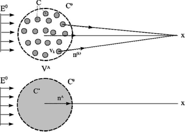
Fig. 1. The scheme of the Maxwell approach to the homogenization problem

Assume that the fi eld E_i ⁰ applied to the medium is constant. The presence of the inhomogeneous sphere V ^A disturbs the applied fi eld E_i ⁰ that can be evaluated by two different ways. First, the far fi eld induced by the small spheres is presented as

N

4nc0 k=1 Vk       x - x| where vk is the region occupied by the k-th sphere. The sum in the right-hand side can be calculated if the fields inside the inclusions are known. To find these fields let us consider each small sphere as a single one subjected to the external field Ei0 . In this case, the fields inside the spheres are constant and determined by Eq. (2.11). Hence, far from the center of the large sphere V A, the sum in Eq. (2.12) is as follows

E ' = —J X ( 5. - 3 n^(k ) n ^{( k} )) 3⁽ c c ^o) E °, i 4 n £ R_k ^{3 (} ” i ” ) 2 c 0 + c ” ,

( k )

n(k) = R-, i Rk ,

(2.13)

v = n a .

Here R_k is the distance from the observation point x and the center of the sphere v_k . Because all the small spheres are practically at the same distance from the far-distant observation point x , R_k ≈ R_A , where R_A is the distance between x to the center of the large sphere V ^A , we have

E'. « Nv(5. - 3 n^An^A) ³⁽ c c ^o) E °, n^A '    4 n R 3 ⁽ ”     ’ ^{j )} 2 c + c j ^,    '

A

^{R i} . (2.14)

R A

Second, the disturbance of the far fi eld by the large sphere V ^A may be treated as the fi eld disturbance of a homogeneous sphere V ^A with an effective conductivity c ^*. The disturbance caused by such a sphere at the same point x is

E ' = —— ( 5. - 3 n^An^A\ ³⁽ c - c ⁰) E °. (2.15) ' 4 n R ” i ”’ 2 c ₀ + c * ”

Equating the disturbances E_i ^' and E_i ^'' in Eqs (2.14) and (2.15) we derive the equation for the effective conductivity c ^*

p(c- co) = c *- cо        Nv c + 2 c0 c * + 2 c 0, p V "

(2.16)

The solution of this equation with respect to c^* yields

C_ = 1 + ² p P   e = ^c - ^c 0

^c 0     ^{1 -} Р^в ’       ^{c + 2 c} 0 ^.

(2.17)

The latter coincides with well-known Clausius-Mossotti equation (in dielectric context) or MaxwellGarnet equation (in conductivity context), and also Lorenz-Lorentz’s equation (in refractivity context).

An obvious drawback of Maxwell scheme is that each sphere is considered as a single one subjected to the external field Ei0 applied to the medium. Strictly speaking, Eq. (2.11) is correct only in the di- lute limit p << 1. In spite of this, equation (2.17) coincides with the expression for the effective conductivity of the composite with random set of spherical inclusions derived by the effective field method that takes into account interactions between the inclusions (see, e. g., [2]).

Note, that using the integral equation (2.8) instead of the differential equations (2.1) allows extending the Maxwell scheme to the case of the composites with anisotropic matrices and ellipsoidal anisotropic inclusions. Let the region V in Eq. (2.11) be ellipsoid with semi-axes a ₁, a ₂, a ₃. If x ∈ V and E_i ⁰ is constant, the field E_i inside V is also constant and is determined by the expression:

E . =(3 ” + A_it ( a ) C k, )^{- 1} E j . (2.18)

Here A_ij ( a ) is the tensor with constant components that is presented as an integral over the unit sphere Ω in 3D-space:

kk

" ” ( a ) = — j K * ( a - k ) d Q , K ” ( k ) = —^ j -, (2.19)

4 n q                     k C k

Q                                  m mn n where Ki*j(k) is the Fourier transform of the kernel Kij(x) in Eq. (2.11); k is the Fourier transform parameter; a = (aij) is a linear transformation that converts the ellipsoid V into a unit sphere. For an isotropic host medium, tensor Aij(a) has the symmetry of ellipsoid and its three principal components have the form:

A k = ^a ₁ ^a 2 ^a 3 j---------- ^{d z}                 , (2.20)

2C0 0 (ak + Z)л/(a 12 + Z)(a22 + Z)(a32 + Z)

( k = 1, 2, 3 ) and are expressed via the standard elliptical integrals.

Application of the Maxwell method to the case of ellipsoidal inclusions yields the following expression for the tensor of the effective conductivity C ^* :

C * = C ⁰ + cP, ( 5. - cA_HP. )^-1,       (2.21)

ij ij ik kj kl lj ,                      .

where

P k =        (v ( a ) C ,m ( 5 mk + A_ml ( a ) C ,1_t Г \

^{v ( a )}                                   (2.22)

v (a) = jna 1 a 2 a 3, and the averaging is performed over the ensemble distribution of the ellipsoid semi-axes, their orientations and orientation of their principal anisotropic axes; tensor Aij is determined by the same formula (2.19) where the transformation aij is the identical one (aij = δij).

In considered examples, a spherical form of the region VA was accepted. It was mentioned in [1] that taking VA in the form of an ellipsoid it makes it possible to describe the properties of a broader class of the composite materials. But the choice of the ellipsoid aspects is not unique. In other words, possibility to vary the form of the region VA demonstrates case, the integral Aij in (2.19) is calculated in the explicit form

A, = A A + A 2 mm j

(2.25)

ambiguity of the Maxwell scheme. But for some cases, this choice of aspects of the ellipsoidal region V^A may be justified.

Let us consider a composite with isotropic ellipsoidal inclusions of the same orientation (Fig. 2).

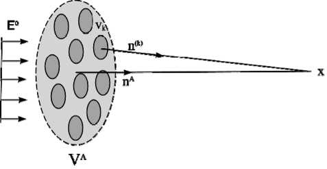
Fig. 2. The Maxwell scheme for the medium with ellipsoidal inclusions of the same orientations

a =

I

A 3

2 C 1⁰1

Y C L aJ A+ 1 2 C 01 I A -1,

A = 1 1 - A -33 ⁰

V                ii

^^^^^^»

,

,

(2.26)

= ( ya ) ² Г 1

^^^^^^B

i.

(2.27)

In spite of isotropy of the matrix phase the macro properties of the composite will be anisotropic. It seems reasonable to take for the region V^A not a sphere but an ellipsoid which aspect ratio and orientation coincide with those of the inclusions. In this case the Maxwell scheme leads to the following expression for the effective conductive tensor

C ij = C o + P C k [ 5 ■ (1 - P ) A ( a C J" ¹ . (2.23)

Again, this equation coincides with ones obtained by other homogenization methods in which the interactions between inclusions were taken into account.

Let us consider, for example, transversely isotropic medium with the property tensor in the form

C 0 = C ° 6 + C 0 m m,, 6 = 5 - m m, , (2 24) ij 11 ij 33 i j ij ij i j ^.

where m_i is the unit vector along the isotropy axis. The medium contains a set of identical spheroidal inhomogeneities ( a ₁ = a ₂ = a , a / a ₃ = γ ) and all spheroid semi-axes a ₃ are directed along the vector m_i (the x ₃ – axis). We assume additionally that material of the inclusion is also transversely isotropic with symmetry axis coincides with semi-axis a ₃. In this

And general formula (2.23) gives the following expression for the components of the tensor C_i ^* _j

C * = C * 0 , + C *3 mm , ,

C *1 = C 11 + pC 11 [ 1 + (1 - p ) AC 11 ]^{- 1},

C 11 = C 11 - C 101 ,

C * = C 3з + pC 3з [ 1 + (1 - p ) A 2 C 3з I"¹,     ^(2.28)

33        33        33 .

Note, that these expressions are also valid for complex λ .

CONCLUSIONS

It is shown that the Maxwell method allows deriving the well-known equations for the effective conductive properties of the composite materials in the most simple and straightforward way. Nevertheless, the method contains an ambiguity connected with the choice of the shape of the region V^A . This ambiguity cannot be avoided in the frame of the method itself. This defect is overcome in the self-consistent effective field method developed in [2]. In this method, the tensor A(a) in Eq. (2.23) is defined uniquely by the correlation function of the random set of inclusions. This correlation function is additional and important information about the random field of inclusions in the composite.