Generation of analysis ready data for Indian Resourcesat sensors and its implementation in cloud platform

Published Online June 2019 in MECS DOI: 10.5815/ijigsp.2019.06.02

• I.    I NTRODUCTİON

  The influence of remote sensing on human lives has seen a magnificent increase in the past decade. From weather predictions to finding the change in habitation of a region over time, it finds application in all walks of our daily life. According to a recent study by the Goddard Space Flight Center, there are approximately 2271 satellites in orbit. This scenario demands the players to be continuously maintaining high standards and redefining themselves from time to time. In this regard, the Indian Remote Sensing (IRS) program of Earth observation has witnessed quantum jumps since its inception in 1988, facilitating India's collection of large

scale multi-spectral data around the globe for various kinds of cartographic, disaster management and resource planning activities.

With the challenging developments in space technology, space is an equally competitive platform as land and water. The massive number of satellites being launched worldwide has opened up a new avenue in investigating earth and other planets of the solar system. Data transmitted from these satellites has seen a exponential increase in terms of data rate and volume. This has necessitated significant advances in image processing in terms of advanced algorithms, improved processing techniques and data storage.

Analysis Ready Data (ARD) is the new paradigm, which can be the new workhorse for application scientists. It is often observed as an obligatory need for application scientists to replicate similar processing steps for the same data , time and again, resulting in huge wastage of valuable scientific resources. The Committee on Earth Observation Satellites (CEOS) define ARD as “satellite data that have been processed to a minimum set of requirements and organized into a form that allows immediate analysis without additional user effort and interoperability with other datasets both through time and space"[ 1,2,3]. This development will ensure an improved access to satellite data and in turn will open the door to a wider audience to exploit it, in addition to servicing existing users with better efficiency and at reduced cost.

The immediate solution offered by technology for all the above stated challenges is Cloud Computing. To harness the flexibility, efficiency and strategic value of Cloud Computing platform, satellite data storage and processing can be envisaged in the cloud platform. In addition to the concept of data storage on cloud, we also need to plan for the entire data processing chain over a cloud platform. This ensures remote access to the huge volume of data and on-demand generation and dissemination of all the required products for analysis or application ready use. The Platform as a Service (PaaS) is a platform based service which allows its users to build, run and deploy its applications without worrying of infrastructure management. The use of this platform will allow us more versatility, cognizance and edge over all the present competitors in the global market. Since cloud computing allows access to all required applications through the internet, it offers very high flexibility in data dissemination to the users. This not only provides a faster and reliable producer side support to the customers but also, helps them build stronger relationships. This paper highlights the design methodology of ARD implemented for Indian Remote Sensing Satellites and its implementation in Cloud Computing Platform.

• II.    Related Work

  The United States Geological Survey (USGS) has processed all of the Landsat 4 and 5 Thematic Mapper (TM), Landsat 7 Enhanced Thematic Mapper Plus (ETM+), Landsat 8 Operational Land Imager (OLI) and Thermal Infrared Sensor (TIRS) archive over the conterminous United States (CONUS), Alaska, and Hawaii, into Landsat ARD. Provision of pre-prepared ARD is intended to make it easier for users to produce Landsat-based maps of land cover and land-cover change and other derived geophysical and biophysical products. The ARD are provided as tiled, georegistered, top of atmosphere and atmospherically corrected products defined in a common equal area projection, accompanied by spatially explicit quality assessment information, and appropriate metadata to enable further processing while retaining traceability of data provenance[4]. The Planet Lab is dedicating a lot of resources and thinking about how to make it easier for user community to bypass preprocessing steps and dive to analysis[5]. Committee on Earth Observation Satellites (CEOS) is developing a Data cube architecture that depends on CEOS analysis Ready Data for Land (CARD4L) to allow immediate analysis and improved interoperability among datasets. Since 1988, NRSC has acquired large volume of multisprectral data from IRS Satellites and propose to generate ARD products for user dissemination.

• III.    Methodology

• 3.1    ARD Products Generation

• 3.1.1    Generation of Radiance Values

Indian Remote Sensing Satellites Resourcesat-2/2A are having a Linear Imaging Self-Scanning Sensor (LISS-III) with a spatial resolution of 23.5 meters providing four spectral bands i.e. Band 2 (green), Band 3 (red), Band 4 (near infrared) and Band 5 (short wave infrared)[6]. The raw data acquired from the satellite undergoes both radiometric and geometric corrections to generate terrain corrected products, ready to be delivered to the user community.

This section describes the methodology adopted for generation of Analysis Ready Data(ARD) products. Fig.1 depicts the flow of ARD products generation. In this activity, the focus is on the generation of Analysis Ready Data products for any scene for Resourcesat 2 /2A, based on demand. Any ARD product is designed to have scene wise terrain corrected product, Top of Atmosphere Reflectance (ToA) for each band, Normalized Difference Vegetation Index (NDVI), Enhanced Vegetation Index (EVI) and a cloud mask band.

The generation of Top of Atmosphere Reflectance starts with the computation of the radiance values of all the bands. The consequent step in the generation of ToA product is the generation of cloud mask[7] and its application on ToA reflectance bands. The product may or may not have a number of cloudy/cloud shadowed pixels, which have to be masked to provide valid product to the user. The masking value is chosen as 255 for cloud and cloud shadow regions.

The ARD product also comprises of NDVI and EVI products of the corresponding scene. NDVI and EVI are computed from the Surface Reflectance of the corresponding bands. This is achieved by subjecting the radiance values to DOS (Dark Object Subtraction)[8]. After the DOS correction,the resultant image would be atmospheric haze corrected which is then applied for calculation of other ARD products. In this process BAND4 (NIR band) and BAND3 (Red band) are considered as inputs to generate NDVI and EVI. Cloud mask is applied to the resultant image so as to get rid off all the cloudy pixels and generate a valid product to the user.

For generating ToA reflectance, radiance values are to be estimated, which is a direct measure of radiance reflected from the surface, neighboring pixels and clouds depending both on illumination as well as the position and orientation of the target. The formula (1) for getting radiance of a single pixel is:

LX = ^{(LmaA Lmin}^  * (Qcal - Qcalmin) + LminZ   (1)

(Qcalmax- Qcalmm)  4                  7             v 7

Where,

L _x = the cell value of radiance

Qcal = digital number (or pixel value)

Lmin _x = spectral radiance scales to Qcalmin

Lmax x = spectral radiance scales to Qcalmax Qcalmin = the min quantized calibrated pixelvalue (= 0 in our case)

Qcalmax = the max quantized calibrated pixel value (= 1023 in our case)

• 3.1.2    Generation of Top of Atmosphere (ToA) Reflectance

Top of Atmosphere (ToA) Reflectance provides us the ratio of radiance reflected to the solar radiation incident on a given surface and is a unit less quantity. For computing ToA reflectance, radiance to ToA conversion [9] is applied to evaluate the ToA of the corresponding spectral band:

Where, pA = Unit-less planetary reflectance

L λ = spectral radiance (from the earlier step) d = distance b/w Earth-Sun in astronomical units ESUN λ = mean solar exo-atmospheric irradiances 6 s = solar zenith angle

Furthermore, the formula for calculating d:

d = (1-0.01672*cos (radians (0.9856*(Julian Day-4))))

Where, Julian day = Total integer no. of days elapsed

-       (7T*LX*d ^

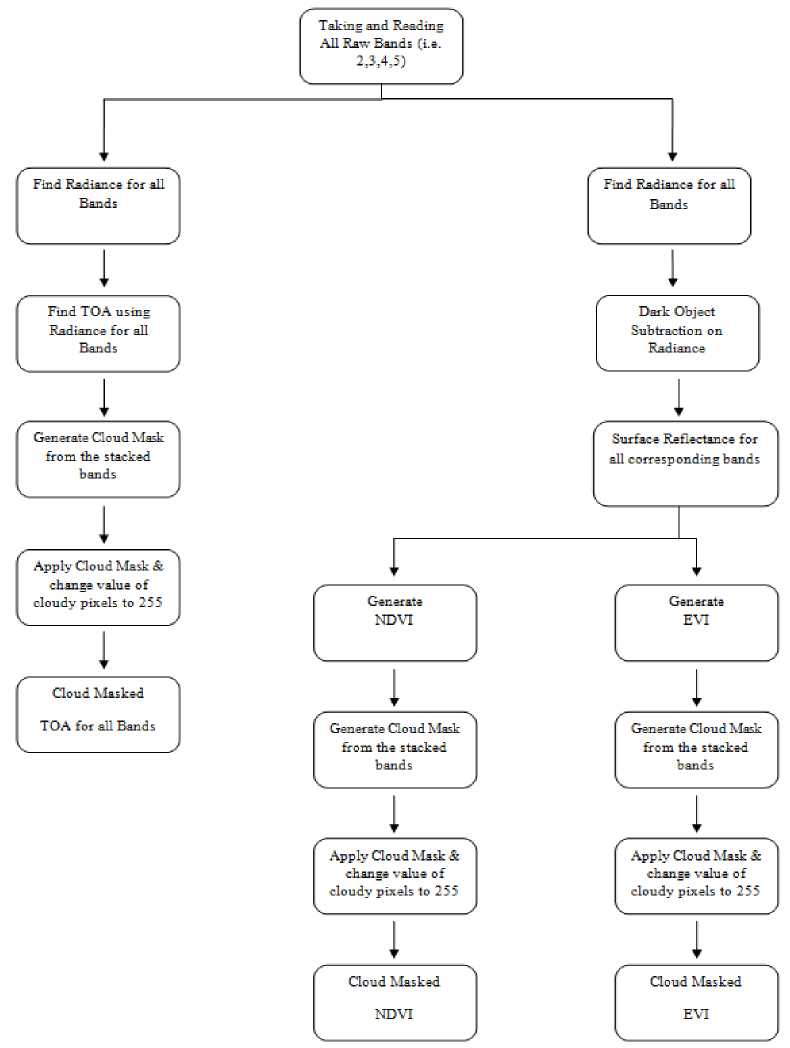
Fig.1. Process Flow ARD

• 3.1.3    Generation of Cloud Mask

• 3.1.4    Generation of Normalized Difference Vegetation Index

Clouds play an important role in the climate system having importance in energy balance of the atmosphere. The data acquired by optical remote sensors is affected by the presence of clouds. In such scenarios, it is very essential to provide information on cloudy pixels for proper and efficient utilization of data. Exact evaluation of cloudy and cloud shadowed pixels is an important pre-processing step for any reliable cloud removal or masking algorithm[7]. Due to the absence of thermal band for Resoursesat-2, an algorithm based on unsupervised classification exploiting spectral attributes is developed by NRSC for automatic cloudy and cloud shadowed pixels detection. Some of the salient features of this utility are – it generates cloud and shadow mask file for each input data, it can delineate snow and moisture cloud, salt pans and moisture cloud which have same spectral signature.

Normalized Difference Vegetation Index (NDVI) is a measure to help us observing the vegetation index of the Earth's surface. It is beneficial in assessing the vegetative cover by employing time series analysis. Its values generally range from -1 to 1. Negative values of NDVI (values approaching -1) correspond to water. Values near zero (-0.1 to 0.1) typically correspond to barren areas of rock, sand, or snow. Lastly, low, positive values represent shrub and grassland (approximately 0.2 to 0.4), while high values indicate temperate and tropical rainforests [8]. The formula for calculating NDVI is expressed below:

NDVI =

(NIR-Red)

(NIR+Red)

Where,

NIR = Band4 (near infrared band)

Red = Band3 (red band)

• 3.1.5    Generation of Enhanced Vegetation Index

  Enhanced Vegetation Index (EVI) can simply be termed as optimal NDVI , where the variations in solar incidence angle, distortions in reflected light caused due to particles of air, canopy background signals and atmospheric conditions are corrected . While, NDVI can show varying results within a time difference of mere 2 hours due to changes in solar incidence angle, shadows and soil boundaries. EVI on the other hand, provides better consistency. The formula for calculating EVI (when blue band is not available in the sensor) is expressed below[9](Jiang et al. 2010)

• 3.1.6    Generation of Surface Reflectance Product

EVI = 2.5 *    ^(NIR-Red)              (4)

(NIR+2.4Red + 1)

The Dark Object Subtraction (DOS) method is an image-based technique to cancel out the haze component caused by additive scattering from remote sensing data (Chavez Jr, 1988). While calculating SR, we first get Lmin as the minimum radiance pixel value. From Lmin, Lpath is calculated as shown below in equation (5) which is then subtracted from all the radiance pixels for DOS correction. After then, SR values of every individual pixel is found by applying the formula shown in equation (6):

L path ^ min ^

_(^ sensor ^ path^)d2

P      E₀cosqz_zT_z

Where, p = Unit-less surface reflectance

Lsensor = is at-sensor radiance d = distance b/w Earth-Sun in astronomical units

E λ = mean solar exo-atmospheric irradiances (B2=184.0; B3=155.1; B4=104.4; B5=22.57) θ z = solar zenith angle (= 90 - elevation angle)

Tz = approximated by θ z

Further more, the formula for calculating d:

d = (1-0.01672*cos (radians (0.9856*(Julian Day-4)))) (7)

Where,

Julian day = Total integer no. of days elapsed

• 3.2    Ard Process Flow

All the ARD products can be ordered by user through the GUI ordering platform for their specific requirements in terms of region, season and spectral bands. The Fig.2 highlights the flow of processes starting from the ordering of data by the user via GUI ordering platform and the subsequent producer's side of receiving the request, processing the raw inputs and sending the resulting ARD data products to the user. The data products generated over the PaaS platform gets stored there and are available to be downloaded by the producer who can then send those to the user either by mail, FTP or any other means according to the request made. There are a number of PaaS platforms available at the market which can be selected according to the languages they support and user interface. As we are using Python as our main language, we selected Python any where PaaS cloud platform which have a great user interface and customer support.

• IV.    Gui Ordering Procedure

The GUI for User Order Processing System(UOPS) allow the users to order ARD data. As soon as the user makes a request (fig.3), a confirmation message pops up to the user with an email notification. The request includes the user's name, email address, date of the data required, corresponding ARD data products required and the satellite name of whose data is needed.

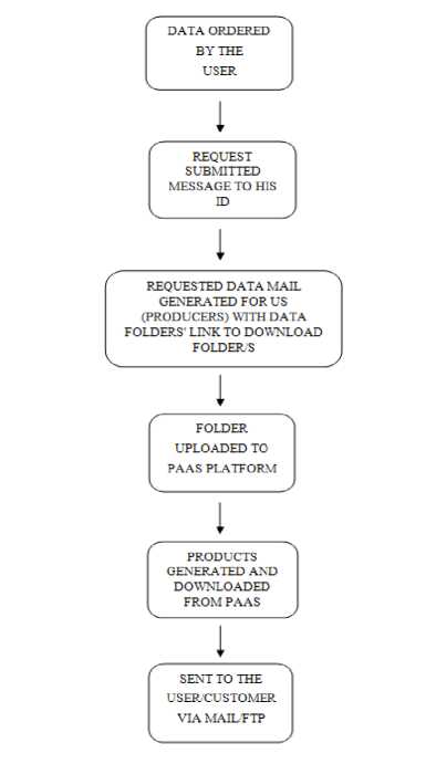
Fig.2. Data ordering and sending process flowchart

The GUI platform also gives option to the user for ordering a time series data. The time series data form asks for name, email address, start and end dates, ARD products to be generated and corresponding satellites for data. Here, we have two additional options allowing the user for deciding a time series on basis of either lat-long or path-row. Where lat-long corresponds to the nearest scene center latitude and longitude coordinates of the data to be acquired, the path-row corresponds to the satellite's path and row information. For a lat-long selection, an input is picked only when the user inputted lat-long is less than 0.05 degrees of the scene center lat-long. On the other side if a path-row selection is made, an input is picked only when the user inputted path and row matches exactly with the path-row of the data within the date range entered.

The request made by the user is also sent to the producer on email with the name, email, start and end date (single date for single day data), ARD products asked, lat long/path-row values (for time series data), satellite name of whose data is asked and the input folder links.

Bands *

□All Bands

□toa

□ Cloud Mask

□ novi

□ EVI

Date *

Satellite *

□ »S2

□ R52A

□ landsat

• Fig.3. Single data request form

• 4 .1 Cloud Platform Data Generation

Here the input folder links represents the cloud links of the data folders. For e.g. we are using Google cloud here hence, Google cloud link is been generated. As soon as the link is clicked the producer is guided to the folder containing the input data to be used for the generation of the ARD products. These data products needs to be downloaded by the producer to implement them on PaaS cloud platform as shown in the next section.

In our research we are using Python any where cloud platform which is a PaaS cloud platform for generating and storing data products as per requested by the user. A PaaS cloud platform provide Platform as a Service allowing users to deploy, run and manage applications over it without complexity of building or maintaining the infrastructure associated with the same. As continued from the earlier step of downloading the required input data from the cloud storage we are now required to upload the same over the PaaS cloud platform as our input data. This data is then subjected to the programs which generates the corresponding ARD products as per asked by the user. The output files then gets saved to the PaaS platform which are available to be downloaded by the producer who can then send them to the user via email, FTP or any other way prescribed.

PaaS platform dashboard show various options like number of consoles available (here one can run multiple programs at single time) and the versions. Also shows the uploaded files, programs, images and output files in a sample directory. All these can be easily added, deleted, modified or downloaded. Also, any additional packages to be used shall be added here only.

-^-- С | й Secure |

1 |f!/usr/bin/python2.7

• 2    from osgeo import gdal

• 3    import numpy as np

• 5    from PIL import Image

• 6    im = Image.open(’/home/singhaks/img/CldMsk.tif')

• 7    width, height = in.size

• 8    print(im.size)

• 9    print(width)

• 10    print(height)

• 11               ~

• 12    print(^H************\nYour program is running. Wait for next 10 minutes

• 14 # Load file, and access the band and get a NumPy array

16 band = src.GetRasterBand(l)

17 ar = band.ReadAsArray()

18 newar = band.ReadAsArray()

19                                  "

20 # Assign a new raster pixel value

21 #print(ar[303,5484])

22 #print(ar[303,5485])

23 #ar[303,5485] = 0

24 #print(ar[303,5485])

25 1=0

27 j=0

29* for i in range(4268):

30’ for j in range(4268):

• 31 -          if(ar[l][j]--125 on ar[1][j]==50):

• 32              nenar[i][j]=l

33              #print("Total * Xs ••••*•« Zs" X (1, j))

34’         else:

35              newar[i][j]=0

36          j+=l

37 i+=l

41 # Save/close the file

42 #band.WriteArray(ar)

43 #del ar, band, src

45 print("************\nHalf done! 5 more minutes.\n************\n")

• V.    Results

  • 5.1    Generation of Top of Atmosphere Reflectance

• 5.2    Generation of Normalized Difference Vegetation Index

Top of Atmosphere (ToA) Reflectance provides us the ratio of radiance reflected to the solar radiation incident on a given surface and is a unit less quantity.

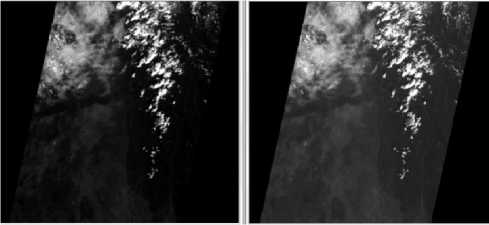
Fig.5. LISS-3 Band 2 and its corresponding Radiance image

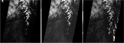
Fig.6. LISS-3 Band 2 image, Radiance,ToA (left to right)

Here, Fig.5. shows the radiance image calculated from the corresponding Band 2 DN image and Fig.6 shows the ToA calculated for the same layer.

Normalized Difference Vegetation Index (NDVI) is a measure to help us observing the vegetation index of the Earth's surface.

The Fig.7 shows the Band 4 (NIR) and Band 3 (Red) which are used to get the resultant NDVI (lower left) which is then corrected with cloud masking. Fig.8 shows the color composite NDVI image in which the green portions depict dense green forests, bright yellow depict shrubs or less dense trees, golden yellow depict grass and magenta or dark blue depict absence of vegetation. Fig.9 shows the level of precision achieved when we use another image for testing which is nearly cloud free. Here it can be observed that pixel level tracing and correction of cloudy pixels is achieved.

Fig.4. Sample Coding Environment

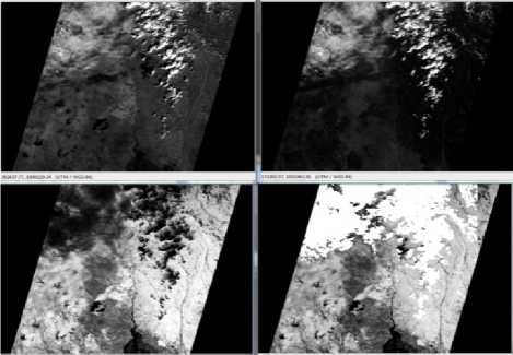
Fig.7. LISS-3 Band 4, Band3, NDVI, Cloud masked NDVI (starting from top left)

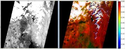
Fig.8. Color Composite NDVI

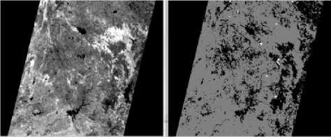
Fig.9. Cloud masking

• 5.3    Generation of Enhanced Vegetation Index

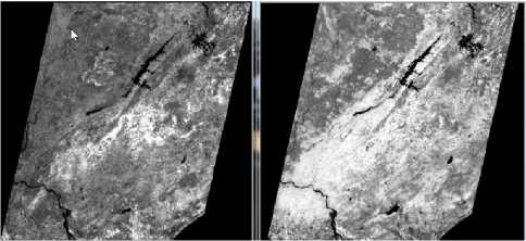
  In Fig.10, the generated EVI is shown using Band4 and Band3 and then cloud masked for cloudy/cloud shadowed pixels. While Fig.11 shows the color composite of the generated EVI image with color strip corresponding to EVI values of the region. The Fig.12 shows a comparison between NDVI and EVI for the same area and time. While the following Table-1 and 2 show the range of NDVI and EVI values respectively. It shows the range of NDVI varying from a minimum of -0.19039 to a maximum of 0.63362. Similarly, for the same region and time the values of EVI ranges from a minimum of -0.25353 to a maximum of 1.2615 (depicting the reason why it is called enhanced vegetation index).

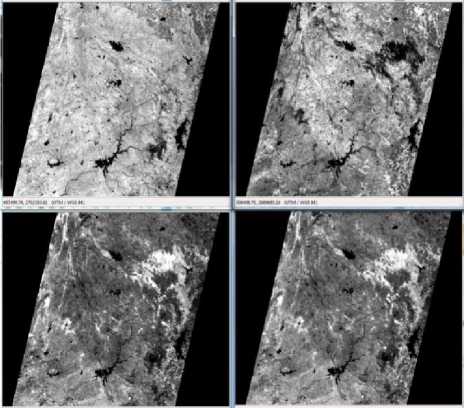
Fig.10. LISS-3 Band4, Band3, EVI, Cloud masked EVI (starting from top left)

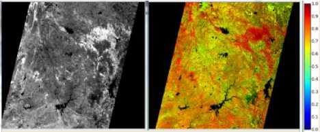
Fig.11. Color Composite EVI

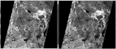
Fig.12. NDVI-EVI Comparison (left is NDVI)

Table-1. NDVI Values range

Width: 7777

Block Width: 7777 Compression: None Pyramid Layer Algorithm:

Height: 7082

Block Height: 1

ErdasBino3 (3X3)

Type: Continuous Data Type: Float Data Order: В IK!

Min: -0.19039            Max: 0.63362 Mean: 0.296

Median: 0.28921 Mode: 0.27312 Std. Dev: 0.091

Skip Factor X: 999      Skip Factor Y:    999

Last M odified:     Wed M ar 2812:36:20 2018

Table-2. EVI Values range

Width: 7777	Height: 7082	Type: Continuous
Block Width: 7777	Block Height: 1	Data Type: Float
Compression:    None Pyramid Layer Algorithm:	ErdasBino3 (3X3)	Data Order: В IK!

Min: 0 25353           Мм: 1 2615 Mean 0 508

Median 0 49215          Mode: 0 44481 Sid Dev: 0.172

Skip Factor X:    999 Skip Factor Y: 999

Last M odified:     Wed M ar 28 12:14:27 2018

• 5.4    Generation of Time Series Data

Time series data analysis provides the advantage of fully capturing the dynamic changes of any pattern viz. vegetation, land cover etc. over a period of time. This helps us noticing the changes in the vegetation index through a course of time varying either due to natural (season changes, natural disaster, etc) or artificial activities (constructions, farming, etc). This data is then implemented for efficient resource planning, strategic and military purposes.

Fig.13 shows a time series NDVI data generated for different dates showing the change in vegetation index over a period of time (approx. 3 years). It is Resourcesat-2 LISS-3 sensor data with Path-103 and Row-060.

19APR2016            08JAN2017

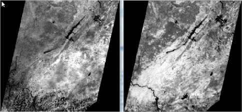
08MAY2017           03JAN2018

Fig.13. LISS-3 Time series NDVI

• VI.    C ONCLUSİONS &  Future Work

We demonstrated the generation of Analysis Ready Data products generation from ResourceSat sensors in this work. The ARD products are accompanied with meta data to ensure processing traceability and queires. Analysis Ready Data (ARD) products has always proved to be a boon to remote sensing satellite data users. It not only facilitates direct usage of data without any additional user effort but also, helps saving a lot of time at customer end. The major benefit of ARD approach is the scalability it offers through adding of new sensors allowing users to focus on EO data analytics. The cloud platform helps producers as well as users for faster data attainability, sharing and research implementations. It allows producers to remotely store, generate and access data and dismiss the dependence over fixed systems. Future work includes creation of consistent time series data, scalability with new sensors, developing inter calibration procedures, data analytics and addition of high security features for cloud data maintenance.

Acknowledgements