Generation of Undistorted Photomosaics of Cylindrical Vesicular Basalt Specimens

Published Online April 2015 in MECS DOI: 10.5815/ijigsp.2015.05.02

Designing and constructing infrastructure assets within rock masses requires samples be obtained through rock coring in boreholes. The sampling assists in developing geologic and engineering descriptions of the rock mass and provides specimens which are tested to determine relevant engineering properties. The samples, known as rock cores, are cylindrical lengths of rock. For geotechnical engineering purposes, the cores range in diameter from 20 mm to 50 mm and the sample length, or core run, is typically 1.5 m. Multiple core runs can be conducted in the same borehole to obtain samples from greater depths. Specimens for testing are cut from core runs. A photograph of multiple core runs is shown in Figure 1. The wooden blocks indicate the length (and thus depth) of the start of each core run.

Photographs of core runs are conducted in accordance with a number of professional standards, for example ASTM D5079 [1] and the US Army Corps of Engineers [2]. According to the ASTM standard, clean cores should be photographed in color with a 35 mm (minimum) camera. For rock samples placed in core boxes, the inside of the box lid should also be photographed. The inside lid should include the appropriate identification as well as a commercially available color strip and a length scale. For boxed rock core that is not particularly sensitive and when preservation of in-situ moisture condition is not required, the core should be photographed in both wet and surface dry conditions. The two sets of photographs help to bring out features that may not be apparent in either surface dry or wet conditions. In Figure 1, the appropriate identification has been removed from the photograph. This type of photograph is acceptable for documenting successive core samples retrieved from drilling operations and may be useful for calculating core based parameters such as core recovery but the scale of the image is insufficient for documenting single specimens.

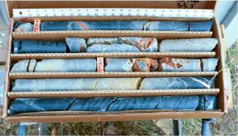
Fig.1. Photograph of core runs

Photographic documentation of rock specimens extracted from core runs is necessary to provide a permanent record of the surface characteristics of specimens prior to destructive testing. The same professional standards that are used for photographing rock cores also provide guidance for photographing rock specimens.

Photographing sections or specimens of core samples is routinely conducted for geotechnical engineering purposes. Schepers et al. [3] describes how core imaging as well as other imaging techniques can be incorporated into geotechnical exploration. The advantage of digital imaging of core sections was first discussed by Trewin et al. [4]. At the time of the Trewin study, there were severe limitations with respect to image resolution, image storage, and distribution of images to other professionals.

These limitations have long since been resolved and core imaging is no longer limited to digital photographs.

There are a number of sophisticated commercial and custom developed whole-core and split-core imaging systems which not only photograph core runs but also perform other imaging and non-destructive testing. These systems have sensors for photographic imaging, X-ray and X-ray CT imaging, hyperspectral scanning, 3D laser profiling, scanning electron microscope capabilities, permeability, electrical resistivity, shear and compression wave velocities, as well as many other measurements. These types of specialty measurements are often used to characterize hydrocarbon reservoir cores, for example Walls and Sinclair [5]. The core imaging capabilities of some commercial firms in fossil fuel exploration and development industries is discussed by Rassenfoss [6].

These sophisticated imaging systems also include image processing and image analysis software. This software is used to provide unwrapped images of core segments or specimens, and various image analyses such as the identification of contacts and discontinuities and the capability to make a variety of measurements from the images. This software may be open-source such as Image-J from the National Institute of Health (for example McMillan [7]) or it may be custom software (for example Beggan and Hamilton [8]).

For routine geotechnical work, images and image analyses provided by sophisticated imaging systems is both cost prohibitive and not required. However, photographs of the core runs does not provide enough resolution for capturing surface features of rock specimens extracted from the core runs. A simple system to provide photographic documentation of core specimens prior to destructive testing would be beneficial.

Such a need arose during a geotechnical engineering study investigating the influence of macroporosity on the physical and engineering properties of vesicular basalt. For the study it was important to retain photographic documentation of the specimens that were tested. Figure 2 contains two photographs of the same vesicular basalt specimen. The vesicles were filled with white spackle to provide a contrast with the dark matrix. The first photograph clearly shows a very large vesicle on the bottom of the specimen surrounded by a somewhat bimodal distribution of large and very small vesicles ranging in shape from almost circular to highly elliptical. The second photograph shows vesicles that are fairly uniform with respect to size and shape. The two photographs could be from two different specimens. This simple example demonstrates that a single photograph cannot successfully capture the surface features of the full specimen surface. Additionally it would be cumbersome to have a series of photographs documenting a single specimen. The best way to fully document the specimens is to obtain an undistorted photomosaic image of the complete specimen surface. A photomosaic is a compound image created by stitching overlapping images of a scene or object [9]. Furthermore, the creation of a continuous photomosaic of a sample surface allows for the implementation of computerized image processing techniques to classify and analyze surface features of the sample.

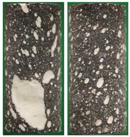
Fig.2. Photographs of opposite sides of the same vesicular basalt specimen

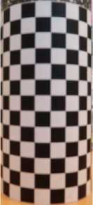
One of the main issues with photographing rock apecimens or any cylindrical object is distortion. Distortion is added to the specimen photographs due to the cylindrical nature of the rock samples. In order to quantify the surface features the removal of this curvature distortion is desirable. Figure 3 shows an example of the curvature distortion obtained by wrapping a flat checker board pattern around a curved cylindrical surface.

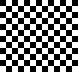
Fig.3. Flat checkerboard pattern (left) and the same checkerboard pattern showing distortion when wrapped around a cylindrical core (right)

This paper describes a series of image processing techniques implemented in MATLAB® to construct an undistorted photomosaic of the surface of a cylindrical specimen from a series of overlapping photographs covering the complete specimen surface. The code has been successfully used to document vesicular basalt specimens.

The remainder of this paper is organized as follows: Section II describes the image acquisition system, Section III discusses the image processing techniques used in this paper, and Section IV contains concluding remarks.

• II.    Image Acquisition System

An automated core specimen photography system named GeoTable was developed for imaging vesicular basalt specimens. The hardware components of the GeoTable system consist of a manual rotary stage that has been retrofitted with a stepper motor and gearing system in order to enable automatic control of the rotary stage. Figure 4 shows an overall system block diagram of the hardware control unit.

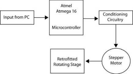
Fig.4. Hardware system block diagram [10]

The custom software application developed to control the GeoTable image acquisition system allows the user to input the number of photographs that will be used to construct the undistorted photomosaic. Figure 5 shows the user-software interaction flowchart for the GeoTable system.

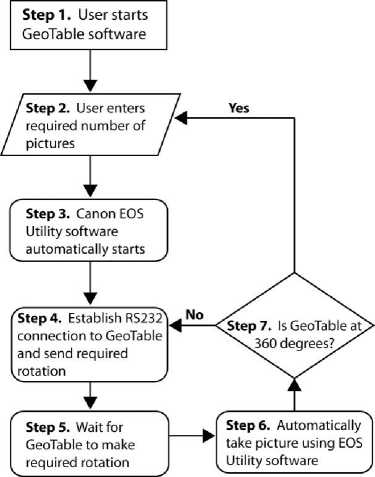
Fig.5. User-software interaction flowchart for the GeoTable System [10]

The software simply divides 360° by the number of photographs to determine the rotation between photographs. The core is photographed using a macrolens against a green screen. This allows for a close-up picture to be taken of the sample which can be easily differentiated from the green background for image processing purposes. For the size of cores used in the study, twenty overlapping pictures of each specimen were adequate to construct a photomosaic. Additional information regarding the GeoTable can be found in Hudyma et al. [10].

• III.    Imaging Processing

A series of four image processing steps are used to create a photomosaic of the rock sample using a sequence of images covering the complete specimen surface. Figure 6 shows the overall flowchart of the four image processing steps.

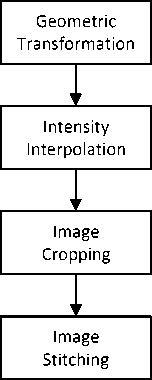
Fig.6. Flowchart of image processing software system

Prior to image processing, the color images obtained from the GeoTable system are cropped using a commercially available image editing program. Since the rock specimen is always in the same location in the image sequence obtained from the GeoTable system, a single cropping mask can be manually placed on the first image and then applied to the remaining images.

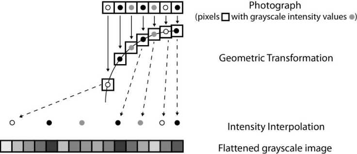
The cropped images are then read into a MATLAB® code where they are converted to grayscale using the rgbtohsv command. The converted images are then subjected to a geometric transformation and an intensity interpolation to produce a flattened image. The transformation and interpolation are shown graphically in Figure 7 and are described below in greater detail. The techniques are adapted from Apostol and Mnatsakanian [11] and Gonzalez and Woods [12].

• A.    Geometric Transformation

The geometric transformation inverts the projection of the cylinder’s curved surface onto the photographic plane during image acquisition, the geometry of which is shown in Figure 8. The optical axis of the camera is through the geometric center of the specimen and aligned along the zero-degree radial line in a cylindrical coordinate system. The projection maps any position on the cylinder’s surface that lies an arc-length of x ’= rθ away from the optical axis to a (horizontal) position x = r sin θ away from the image’s center. Eliminating angle θ from the previous equations, the identity x = r sin( x ’/ r ) can be obtained.

Photograph (pixels □ with grayscale intensity values •)

Geometric Transformation

Intensity Interpolation

Flattened grayscale image

о

Fig.7. Geometric transformation and intensity interpolation to obtain a flattened grayscale image

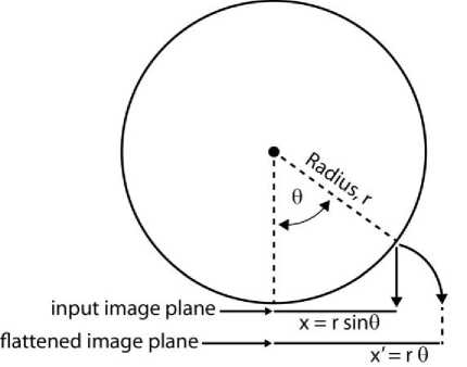
Fig.8. Geometric transformation (after Apostol and Mnatsakanian, 2007)

spatial positions in the image plane are given by Equation 1.

x =

2 r ( M-1) u -M-1(    2 J

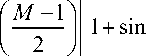
The desired “flattened” image, on the other hand, will consist of horizontal pixels that cover an arc-length equal to half the circumference of the cylinder, or n r . Let M’ denote the number of horizontal pixels of the flattened image, as M in proportion to the ratio of the halfcircumference and the diameter i.e.,

M' = round

During the image capturing stage, the camera is located at a sufficient distance from the specimen in order to make the assumption that surface positions at angles between -90 degrees and +90 degrees (corresponding to the far left and far right edges of the input image) are visible. Moreover, the projection of the sample into a linear image is symmetric about the zero degree axis and the required amount of projection increases with increasing arc length.

The input image (after cropping the background and performing a gray-scale conversion in MATLAB®) consists of M horizontal pixels, covering a spatial distance in the image plane equal to the diameter of the cylinder, or 2 r . That is, if each pixel of the input image is indexed with integers u = 0,1,…, M -1, the corresponding

Indexing each pixel of the flattened image with integers u’ = 0,1,…, M’ -1, each corresponding arc-length position along the cylinder’s perimeter is given by the formula

x' =

it is found that:

n r

2  ( , M '-1)

2 u -

M'-1 (     2  )

Employing the identity x = r sin

, and equating,

Row of pixels in the input image

Intensity Interpoloation

N-----►■◄—►

u

Fig.9. Intensity interpolation scheme

x

r

2 Г M - 1 ) u -

M - 1 (     2   )

= sin

n

2 Г . M '— 1 )

2 u -

M '- 1 (      2   )

= sin

x ' r

From Equation 4 it follows that the value u in the input image associated to each pixel location u’ in the flattened image is given by the formula

2 Г , M '- 1

2 u ^-

M ‘-11      2

where u ’=0,1,…, M ’-1.

Due to the appearance of the sin function, the values of u from this expression will almost always be non-integer. However, the input image has a well-defined pixel intensity only at integer locations u = 0,1,…, M -1. Thus, some non-ambiguous rule for estimating the grayscale intensities between two pixels of the input image is required.

• B.    Intensity Interpolation

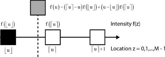
The geometric transformation derived in the preceding section, relating a specific (horizontal) pixel location u’ in the flattened image to the location u in the input image, results in non-integer values for u and thus requires a rule for estimating intensity between integer-valued pixels. A standard intensity interpolation technique is employed that computes the weighted average of the two pixel intensities in the row direction that surround location u. More precisely, for a given row of the input image, let f( z ) denote the normalized grayscale intensity and z denotes the horizontal integer valued pixel location which can range from 0 to M -1. The intensity associated to any realvalued location u in [0, M-1] is given by the formula

f (u )=(Гu "I-u) f (Lu _l)+(u-Гu "I) f (Гu "I)    (6)

where r u 1 and L u J denote the ceiling and floor, respectively, of the real value u . Figure 9 is a graphical representation of the intensity interpolation scheme.

• C.    Image Cropping

Figure 10 is the resulting input image which has been geometrically-transformed and intensity-interpolated. It can be observed that while the curved sample surface is still observable towards the sides of the image, the center portion of the image has been transformed into an undistorted image.

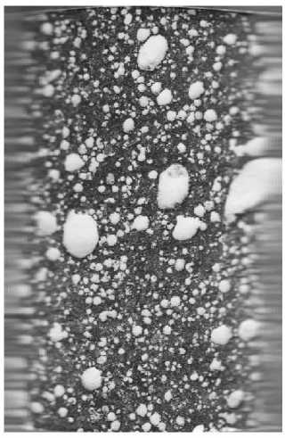
Fig.10. Image after the geometric transformation and intensity interpolation algorithms

Since the system is designed to take multiple images around the core surface, the distortion at the sides of the image can be eliminated by re-cropping the geometrically-transformed, intensity-interpolated image and keeping only the center portion of the image. The second cropping is implemented by defining a range of pixels to keep in each row of the image. A maximum differential is defined based on the dimensions of the image which is then cropped to an equal size on either side of the image center line. This second cropping leaves an unwrapped image without any distortion as shown in Figure 11.

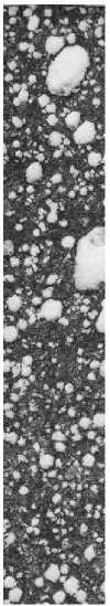
Fig.11. Cropped image.

• D.    Image Stitching

The final step in producing a complete photomosaic image of the specimen surface is stitching together all of the geometrically-transformed, intensity-interpolated, cropped images. This process is depicted in Figure 12.

The photomosaic image is generated by vertically aligning the first two cropped images. The second image is then passed horizontally over the first image in single column increments. After each column step, the crosscorrelation between the two images is compared to a user-defined threshold. The cross-correlation provides a numerical value to explain the level of match between the columns of each image. If sufficient cross-correlation exists between the images, the two images are then considered a match. Overlapping pixel values are then averaged between the two images to create a new image that combines the first two images. This process is then repeated for the remaining images.

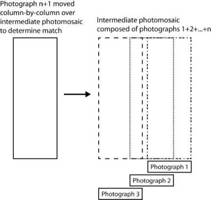
Fig.12. Stepwise progression of photostitching to develop a photomosaic

After all of the images of the core surface have been stitched to form a photomosaic, the left and right sides of the image will exhibit a certain amount of overlap. This unnecessary overlap is eliminated by cross-correlating the two ends of the image in a similar pixel by pixel manner and then cropping both sides of the image at the point at which they meet. The resulting final photomosaic image is a complete undistorted 360 degree photograph of the specimen surface, as shown in Figure 13.

It should be noted that this cross-correlation method for image stitching requires sufficient intensity variation between pixels in each vertical column of the image. This technique is particularly well suited for vesicular basalt specimens. This technique may not be appropriate for photomosaic development in other specimen lithologies.

• IV. Conclusion

A technique to transform a series of overlapping images of a prepared cylindrical rock specimen to a single undistorted photomosaic of the complete specimen surface is described and implemented in MATLAB®. Color photographs are cropped to isolate the specimen from the green screen background. The images are converted to grayscale and a geometric transformation and intensity interpolation is applied. The result of the transformation and interpolation is a series of flattened images. The flattened images are cropped a second time because they are still highly distorted near the edges. The cropped photographs are then stitched using a crosscorrelation algorithm. Finally the image is tested so that the two edges correspond to each other. The result is a complete 360 degree undistorted photomosaic of the surface of a cylindrical specimen.

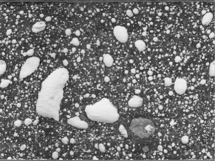
Fig.13. Example of a completed photomosaic

Acknowledgment

The authors would like to thank the Dr. Dean Krusienski from Old Dominion University for his guidance in the development of the MATLAB code and Kevin Nguyen for helping to annotate the original MATLAB® code. The photograph in figure 1 was provided by Dr. Jeffrey Keaton, National Geotechnical Practice Leader for AMEC. The basalt cores were provided by Dr. Mary MacLaughlin and Brian Kuhn of Montana Tech of the University of Montana, Department of Geological Engineering.