Genetic Algorithm to Solve the Problem of Small Disjunct In the Decision Tree Based Intrusion Detection System

Published Online July 2015 in MECS

Today we are living in the digital era and the alot of finance is being invested by the individuals and the organizations for fulfilling their need and wants, that’s why computer network is the most important foundation in the today’s era. Intrusion detection is the process to finding out attack in the computer network infrastructure by exploring the network packets or the TCP/IP packets. IDS is the suitable tool to overcome the security problem in the network infrastructure. There are so many applications such as firewall, access control, antivirus, anti-spammer etc. are availing the security but are not to provide 100 percent security to the network resources [1]. One reason behind this is the most of the security equipment’s are based on the data patterns and they required, time to time fine tuning to escape from the cope of the network attacks. Today innovation in the science and technology, every day size of the network data expanded exponentially and the manual analysis of these is almost impossible [2]. So there is a need of automatic attack detection system which can possibly extract useful information from the network data which is possibly unknown.

An intrusion detection system or simply IDS is a hardware or software or both that attempt to detect malicious activity in the Internet or World Wide Web. The intrusion detection system (IDS) can be categorized into two categories namely anomaly detection and misuse detection [33-36]. Misuse detection system is ability to detect malicious activity in the computer network against the known malicious activities. In other words we can say that misuse detection system are based on the attack pattern and if any upcoming packets fall with the existing results or signatures is treated as the attack otherwise treated as normal traffic. This is very difficult to maintain the rule base for all types of attack or network vulnerabilities, they required timely updation. In anomaly detection system the administrator of the system define the various cases of normal pattern, if any of the upcoming packet violate this, is treated as anomaly. This is very difficult to maintain, it’s because if the any of the normal user uses the system resources or network resources in a different way, is treated as an anomaly. It may have the high false alarm rate [3, 4, and 5].

Development in the data mining or machine learning, the intrusion detection system were developed from the automatic extraction of the rules besides the human experts. Today there were a lot of system were suggested by the researchers for generating the IF-Then rules without the help of human experts like decision tree, fuzzy rule based system etc. Data mining is the interdisciplinary field which can be used to extract knowledge from the large collection of data, in other words we can say that it will discovering rules that are possibly unknown.

The intrusion detection system which are based on the rule base are biased towards the small disjunct. This is due to the given preferences to the specialization rather than the generalization. Hence the large disjunct are given preferences in the rule based systems as compared to the small disjunct. The large disjunct are the rule sets which covers a large number of training instances and small disjuncts are the rules sets which covers small number of the training instances. The rule induction methods ignores small disjunct and discovers only large disjunct therefore the classification accuracy will significantly degraded in many circumstances [8, 9, 10].

In this paper a decision tree and genetic algorithm based intrusion detection system is presented. The basic idea is, rules that are discovered through decision tree algorithm and the rule set which are belongs to small disjunct are fine-tuned using the meta heuristic genetic algorithm, after the rule optimization the optimized rule and the rules discovered by the decision tree which are large disjunct rule set are combined to model a hybrid intrusion detection system. System developed using decision tree and genetic algorithm (DTGA) is best in in comparison to many other existing systems. Contribution to this paper are: (1) the proposed decision tree and genetic algorithm based intrusion detection system have the capability to handle the noise or outlier. (2) The proposed intrusion detection system is not cope with the problem of small disjunct. (3) System is adaptable in nature. (4) Automatic extraction of the rules from the large volume of data without any human intervention. (5) Can detect anomaly as well as the misuse type of intrusion. (6) Proposed intrusion detection also uses the rule pruning system to discover simplified candidate rule, unnecessary or low information gain conditions are removed from the rule antecedent.

• A.    Need of Intrusion detection system?

An IDS is network security tool used to detect vulnerable activity in the computer network. IDS works on network traffic from the network resources and then analyses it for possible vulnerability or anomalous network traffic detection [6, 7]. IDS can monitor or analyses the activity of the user in the computer network for auditing the network anomaly or misuse in the network. It can also perform the statistical analysis of the network activity from the already existing normal or anomalous patterns of database to detect the vulnerability. Need of the intrusion detections are given below:

• a)    To maintain the integrity, reliability, confidentiality and availability of the network resources.

• b)    To build a robust security system for individuals or organizations, so that non-expert employee can possibly be the part of the security management system.

• c)    To help the security administrator to make the security policy for the organization.

• d)    To detect vulnerable activity which May anomaly or misuse to the network infrastructure.

• e)    To automate the network monitoring activity.

• f)    To tracing out the activity of the users of the network resources and if the user is anomaly then prevent from it.

• g)    To monitor the network activity without human intervention.

• B.    How data mining is helpful in network security?

• a)    The attack signature developed based on the new malicious network vulnerabilities, the validity of the signature depends on the uniqueness and detection rate. The attack code can changed to

make new vulnerabilities easily and the manual analysis of it is very difficult.

• b)    The size of the data in Internet is growing exponentially, and the manual analysis of it is approximately impossible. Manual analysis of network data is possible but it will take too much time, finance and the most important thing is it may not be real time system.

• c)    For automatic extraction of the knowledge from the huge amount of the data, the data mining based system are adaptive in nature.

• d)    Data mining also support the rule optimization or the signature optimization, It may be provide the better accuracy in comparison to other parallel system

• e)    The current IDS will generate many false positive it’s because it is very difficult to generate unique signature frequently.

• f)    The most of the intrusion detection or the vulnerability detection systems are rule based system. So through rule based system, which are not automatic and adaptive can’t detect which there are no defined signature. In other words we can say that if signature not written for a vulnerability type there is a chance the system may not detect it as an attack.

• C.    Related work

In [11] Koshal et. al. presented a cascading of c4.5 and SVM to build a rule based IDS. Performance of the proposed model is superior and the system generate low false alarm. The main reason behind cascading of classifiers is to improve the performance of the systems as compared to the single classifier. In [12] Jiang et. al. presented analysis of tree based classifiers on NSL KDD cup dataset, Random Tree method is better in comparison to other decision tree used in this in terms of classification accuracy and error. In [13] an incremental decision tree based IDS is proposed. The decision tree is based on the concept of rough set theory. The prosed system provide the competitive result to the existing systems. In [14] panda et. al. presented a hybrid intrusion detection system using the multi classifier to detect the intrusion. According to authors, instead of single classifier multi classifier system because the multi classifier system provide the superior classification accuracy. In [15] Selvi et. al. presented an intelligent decision based intrusion detection system. This proposed method is based on the concept of Manhattan distance algorithm and for performance evaluation KDD CUP 99 data set is taken. In [16] Senthilnayaki et. al. proposed genetic algorithm and modified J48 based system. In this genetic algorithm is used for feature selection and the modified decision tree algorithm is used for classification. The system is evaluated with the help of kdd cup data set. In [17] Muniyandi et. al. Proposed an anomaly detection model using the cascade kmeans and c4.5. The clustering method K means is used to first partition the learning data into k clusters. Here in this kmeans clustering, Euclidean distance is taken for similarity measure. Applying decision tree c 4.5 on each clusters to refines the boundaries to classify normal and anomaly cluster. Prema et. al. in [18] presented active rule based intrusion detection system, which is enhancement to the C4.5 decision tree method and for performance evaluation kddcup dataset is used. The proposed method give effective performance in classification of intrusion in the computer network. In [19] Mulaye et. al. presented a decision tree and SVM based IDS, which is called Tree structured multi class SVM. The SVM is originally design for binary classification but the proposed model in this paper have the capability to do multiclass classification. The proposed method efficient in terms of training and testing time. In [20] author has proposed a Decision tree based light weight intrusion detection using a wrapper approach for anomalies detection in network. The proposed method has evaluated using detection percentage and the error percentage. The proposed method gave best results among following classifiers: Decision Stump, C4.5, Naive Bayes, Random Forest, Random Tree, and REP Tree.

• D.    Motivation for proposed research work

The classification rules are termed as the disjunction of rules and the each rule are treated as a disjunct. In a rule based system two types of disjunct are found that’s are small disjunct and large disjunct. The small disjunct are the disjunct they covers a small number of instances and the large disjunct covers a large number of instances in the learning set or the training set. Due to presence of the small disjunct the system may be error prone and it will affect the overall accuracy of the system [21-24]. Let’s assume that the small disjunct may cover few examples but the set of small disjunct may cover large number of instances in the training set or the learning set, So that there is a requirement of the system which may recover from the cope of the problems due to small disjunct. The most of the systems are biased towards the discovery of the large disjuncts besides the small disjunct, its natures tendency to give attention to the generalization then the specialization. Network security is very important era today because the alot of finance and the private data are floating in the network in the form of the packets and none of the individuals or organization would compromise with the security of the network resources. So the role of small disjunct in the accuracy is can’t be ignored to compromise the security breaches in the World Wide Web. It’s because the set of small disjunct may covers the large number of learning instances. In such scenario need to required best optimized small disjunct rules in order to get the better classification accuracy rate. So that the security of the system can’t be compromised due to presence of the small disjunct. The proposed decision tree and the genetic algorithm based intrusion detection system handle the small disjunct with the help of the genetic algorithm

• II.    Materials and Methods

This section provides the details of the decision tree and genetic algorithm. In the decision tree section, presents the how decision tree is used to do classification, why decision tree is popular, the basic decision tree algorithm and the popular attribute selection measures available in the decision tree. The genetic algorithm section presents the detail about the GA, GA operations like selection, crossover, mutation, rule pruning etc. And the GA section also describes the how the metaheuristic is used for rule optimization task.

• A. Decision Tree

Decision tree is the decision making tool in the data mining, which is use to do classification task. The decision tree has root node, branches and leaf nodes. The Decision tree has one root node, zero or more branches and zero or more leaf node. The leaf node in the decision tree which is built after training process is labeled with the target class or output and the non-leaf nodes are labeled with the attributes. The branches in the decision tree or classification tree represent the test outcome on the attribute or non-leaf node. The number of branches from the non-leaf node is depend on the tree type and the attribute type and also the algorithm used for the training process. The top most node in the tree is the root node which is the start of the tree. From the above discussion we can say that the decision tree is the collection of the nodes and the branches but here branches may be null but not the node, the tree contain at least one node. Some of the decision tree based classifiers are explained in [25-29].

In data mining , decision tree represent the classification model in the form of the tree like structure. In the training phase the decision tree construction process breaks down a dataset into smaller and smaller subsets and build an associated classification tree or decision tree and this process     grows until the terminating condition is not found. This is the very simple method and it does not depends on any parameters unlike neural networks.

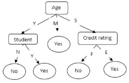
Fig.1. Decision tree

The above given figure 1 represent the decision tree, in this the aim of the tree is to whether a customer buy a computer or not .Each internal node of the classification tree represents the test on the feature or attribute for example age i.e. is the internal node or non-leaf node, here it’s also the root node it has three outcomes as follows young(Y), middle aged (M) or senior (S) similarly credit rating has fair (F) or excellent (E). Each leaf node represents a class, here classes are yes and no.

• a.    How are decision trees used for classification?

• 1.    Given a tuple, X , for which the associated class label is unknown, the attribute values of the tuple are tested against the decision tree.

• 2.    A path is traced from the root to a leaf node, which holds the class prediction for that tuple. Decision trees can easily be converted to classification rules.

• b.    Why are decision tree classifiers so popular?

• 1.    The construction of decision tree classifiers does not require any domain knowledge or parameter setting, and therefore is appropriate for exploratory knowledge discovery.

• 2.    Decision trees can handle multidimensional data.

• 3.    Their representation of acquired knowledge in tree form is intuitive and generally easy to integrate by humans.

• 4.    The learning and classification steps of decision tree induction are simple and fast. In general, decision tree classifiers have good accuracy.

• 5.    However, successful use may depend on the data at hand.

• c.    Decision Tree Algorithm: generate decision _tree.

> Input: D (data set), AL(attribute list), AS(attribute selection method)

> Output: decision tree

> Process:

• 1.    Create a Node N;

• 2.    If tuples in D all are same class C then return N as a leaf node labelled with class C;

• 3.    If attribute list is empty then return with the majority class in D;

• 4.    Apply attribute_ selection_ method (D,AS) to find the best splitting criteria;

• 5.    Label node with splitting criterion;

• 6.    If Splitting attribute is discrete valued and multiway split allowed then AL=AL- splitting attribute.

• 7.    for each outcome j of splitting criterion (partition the tuples and grows sub tree for each partition)

• 1)    Let D j be the set of data tuples in the D satisfying the outcome j;

• 2)    If D j is empty then attach a leaf labelled with class in D to node N;else attach the node returned by generate_decision_tree( D j ,AS) to node N.

• 8.    Return decision tree.

End for.

• d.    Explanation of Decision tree algorithm:

The decision tree algorithm is called along the three parameters data source, Attribute selection measure and the list of attribute. Initially the dataset or data source contains whole training tuples along with the class label, the attribute list here contains the set of attribute that describe the data source and the attribute selection measure describe the procedure for selecting the attribute that best discriminate the training tuples according to the class label. The tree is binary or multiway is depend on the attribute selection measure.

If the Training tuples are all labeled with the same class then a node is crated and is labeled with the class label otherwise according to the given attribute selection measure choose the best splitting attribute subset. The node which is chosen as splitting attribute is labeled with the splitting criteria. A branch is extended from the created node to each outcomes of the splitting criteria.

Three possible cases for outcome of the splitting attribute:

• 1.    The outcome is discrete valued : If the outcome of the splitting attribute is the discrete valued then the branches are created for each known values and is labeled with the value of the attribute. Because the all the tuples have the distinct value its need not to considered in the next iteration. Therefore the attribute is removed for the attribute list.

• 2.    The outcome is the continuous valued : If the outcome of the splitting attribute is continuous valued, in this scenario the outcome have the two possible values A<= splitting node and second one is the A> splitting node. The tuples are partition such that that the D1 subset of D satisfy the first condition and D2 contains the rest or the tuple those who satisfy the second condition.

• 3.    The outcome is the discrete valued and T must be binary tree : In this case the splitting on node is binary valued, In this, to determine the best binary split on A , Each subset, S_A , can be considered as a binary test for attribute A of the form “S _A ∈  ”

Given a tuple, this test is satisfied if the value of A for the tuple is among the values listed in SA . If attribute A has v possible values, then there are2 ^v possible subsets but super set and null set are excluded from the test condition.

• e.    Attribute selection measures:

• 1.    Information Gain: The expected information needed to classify a tuple in D .  .      ()

2. Gain Ratio :

( )=-∑        )(1)

How much more information would we still need (after the partitioning) to arrive at an exact classification . .()

( )=-∑   |  |     (  )(2)

Information gain is defined as the difference between the original information requirements i.e., (based on just the proportion of classes) and the new requirement (i.e., obtained after partitioning on A ).

()=    ( )-      ( )      (3)

SplitInfoA ( D )=-∑ j=i | ^ | log2 ( | | )     (4) GainRatio =        (-)               (5) () 3. Gini Index: Gini ( D )=1-∑i" 1 Pi2          (6) GiniA ( D )= ^Gini ( Di )+ ^Gini ( d2 )      (7) AGini ( A )= Gini ( D )- GiniA ( D )       (8) The measures listed in equation (1) to equation (8) are taken from [37]. f. Decision tree explanation with an Example: Weather Data: Play or not play? Table 1. Example dataset
Outlook	Temperature	Humidity	Windy	Play
sunny	hot	high	false	No
sunny	hot	high	true	No
overcast	hot	high	false	Yes
rain	mild	high	false	Yes
rain	cool	normal	false	Yes
rain	cool	normal	true	No
overcast	cool	normal	true	Yes
sunny	mild	high	false	No
sunny	cool	normal	false	Yes
rain	mild	normal	false	Yes
sunny	mild	normal	true	Yes
overcast	mild	high	true	Yes
overcast	hot	normal	false	Yes
rain	mild	high	true	No

Here Table 1 is the training set for whether paly or not? In this given training set there are 14 training instance 4 attributes and a class attribute. Here problem is how to create a classification tree, which attribute is to select? This problem is solved the help some of the very popular attribute selection measure like information gain. The attribute measure tells which attribute is most suitable for attribute selection. Here information gain is taken as an attribute selection measure to construct a decision tree in the C4.5.table 3-4 shows the calculation of information gain and the figure 2-4 shows the generated decision tree.

g. Information Gain for weather data

Information gain (D) = (information before split) – (information after split)

Table 2. Calculation of information Gain or entropy of whole dataset(D)

Parameter	Outcome (in bits)
Info(D) where D= Weather Dataset	0.940
info A (D) where A = Outlook	0.693
infoД (D) where A = Temperature	0.911
infoД (D) where A = Humidity	0.788
infoД (D) where A = Windy	0.892
Gain(Outlook)	0.247
Gain(Temperature)	0.029
Gain(Humidity)	0.152
Gain(Windy)	0.048

Sunny		[ Outlook |
		/\'^-Overcast *
				Yes (3) No (2)
Yes (2) No (3)		Yes (4) No (0)

Fig.2. Tree generated and Outlook as a splitting attribute

Table 3. Calculation of information Gain or entropy of dataset(D) having outlook=sunny

Parameter (where Outlook =sunny)	Outcome (in bits)
Info(D); where D= All tuples of Dataset D having Outlook =sunny	0.970
infoД (D) where A = Temperature	0.677
infoД (D) where A = Humidity	0.477
infoД (D) where A = Windy	0.968
Gain(Temperature)	0.293
Gain(Humidity)	0.493
Gain(Windy)	0.002

		| Outlook |
Sunny		/\\ Overcast *
Humidity 4_____________________V		Yes (4) No (0)

Hormal

Yes (3)

No (2)

High

Yes	(0)
No	(3)

Yes (2)

Mo (0)

Fig.3. Tree generated and Humidity as a splitting attribute in left most node

Table 4. Calculation of information Gain or entropy of dataset(D) having outlook=rain

Parameter (where Outlook =rain)	Outcome (in bits)
Info(D); where D= All tuples of Dataset D having Outlook = rain	0.970
infoД (D) where A = Temperature	0.968
infoД (D) where A = Humidity	0.968
infoД (D) where A = Windy	0.477
Gain(Temperature)	0.002
Gain(Humidity)	0.002
Gain(Windy)	0.493

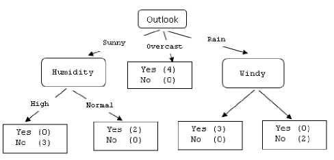
Fig.4. Tree generated and Windy as a splitting attribute in right most node (Final Tree)

Number of Nodes: 8 Number of Splits: 3 Maximum Depth: 2

Rules Generated:

If (Outlook = sunny AND Humidity = high) Then Play? = No (3.0)

If (Outlook = sunny AND Humidity = normal) Then Play? = Yes (2.0)

If (Outlook = overcast) Then Play? = Yes (4.0)

If (Outlook = rain AND Windy = FALSE) Then Play?

= Yes (3.0)

If (Outlook = rain AND Windy = TRUE) Then Play? = No (2.0)

A. Genetic Algorithm

Genetic algorithm is a search based optimization technique and is based on the idea of natural selection. The genetic algorithm is basically used for optimization task. For example in clustering it can be used for cluster center optimization. Data clustering is the data mining task in this the instances are grouped in n clusters based on the similarity between the instances. The basic element of the clustering task is centroid. Genetic algorithm based data clustering idea optimizes the clusters centers up to n generations using the genetic algorithm. Key points in GA are crossover, mutation and fitness evaluation. In GA the candidate solutions are developed near to the enhanced solution using crossover and mutation. [30-32]

The process of the GA is initiated from the generation of the initial population, then this population is evolved iteratively. The population generated through crossover and mutation in each iteration are called generation. In each iteration the fitness of each individuals are evaluated, if the fitness of the newly generated population is better than the previous one then the previous is replaced by the new  generated population otherwise the previous population is kept as it is. This process will continue up to n generation or until stopping criteria matched.

• •    Chromosome: Every living being have a collection of cells. In each cell there is the some chromosomes. Chromosomes are the strings of DNA and serves as model for the whole organism.

• •    Reproduction: During reproduction, first occurs recombination (or crossover). Genes from parents form in some way the whole new chromosome. The new created offspring can then be mutated. Mutation

means, that the elements of DNA are a bit changed. This changes are mainly caused by errors in copying genes from parents. The fitness of an organism is measured by success of the organism in its life.

• •    Encoding: The encoding in GA tells how to encode the individual solution in the proper format for the optimization task. The process of encoding is depends on the problem itself. There are several methods for encoding like binary encoding, permutation encoding, value encoding etc.

• •    Crossover: Crossover selects genes from parent chromosomes and creates a new offspring. The simplest is to choose randomly some crossover point and everything before this point copy from a first parent and then everything after a crossover point copy from the second parent. Figure 5 shows the representation.

Chromosome 1	11011 |00100110110
Chromosome 2	11011 |11000011110
Offspring 1	11011 |11000011110
Offspring 2	11011 |00100110110

Fig.5.Individual representation for crossover

• •    Mutation: After a crossover operation, mutation task takes places. This is to prevent falling all solutions in population into a local optimum of solved problem. Mutation changes randomly the new offspring. For binary encoding can switch a few randomly chosen bits from 1 to 0 or from 0 to 1. The mutation depends on the encoding as well as the crossover. For example when we are encoding permutations, mutation could be exchanging two genes. Figure 6 shows the operations.

Original offspring 1	1101111000011110
Original offspring 2	1101100100110110
Mutated offspring 1	1100111000011110
Mutated offspring 2	1101101100110110

Fig.6. Individual representation for mutation

• •    Termination: The termination in GA tells when to stops the process. Common terminating conditions are:

> A solution is found that satisfies minimum criteria

> Fixed number of generations reached

> Allocated budget (computation time/money) reached

> The highest ranking solution's fitness is reaching or has reached a plateau such that successive iterations no longer produce better results

> Manual inspection

> Combinations of the above

• •    Crossover probability: says how often will be crossover performed. If there is no crossover, offspring is exact copy of parents. If there is a crossover, offspring is made from parts of parents' chromosome. If crossover probability is 100%, then all offspring is made by crossover. Crossover is made in hope that new chromosomes will have good parts of old chromosomes and maybe the new chromosomes will be better. However it is good to leave some part of population survive to next generation.

• •    Mutation probability: says how often will be parts of chromosome mutated. If there is no mutation, offspring is taken after crossover (or copy) without any change. If mutation is performed, part of chromosome is changed. If mutation probability is 100%, whole chromosome is changed, if it is 0%, nothing is changed.

• a.    Why Genetic algorithm?

• •    For Rule optimization.

• •    To increase the classification accuracy.

• •    To solve the problem of small disjunct in decision tree based classifiers.

• •    For finding hidden pattern from large amount of data which is previously unknown.

• •    Easy to implement.

• b.    Basic Genetic Algorithm

Step 1. [Start] enerate random population of n chromosomes (suitable solutions for the problem)

Step 2. [Fitness] Evaluate the fitness (x) f each chromosome x in the population

Step 3. [New population] reate a new population by repeating following steps until the new population is complete

Step 3.1. [Selection] Select two parent chromosomes from a population according to their fitness (the better fitness, the bigger chance to be selected)

Step 3.2. [Crossover] With a crossover probability cross over the parents to form a new offspring (children). If no crossover was performed, offspring is an exact copy of parents.

Step 3.3. [Mutation] With a mutation probability mutate new offspring at each locus (position in chromosome).

Step 3.4. [Accepting] Place new offspring in a new population

Step 4. [Replace] Use new generated population for a further run of algorithm

Step 5. [Test] If the end condition is satisfied, stop , and return the best solution in current population

Step 6. [Loop] Go to step 2

• c.    Explanation of genetic algorithm with current scenario

The main aim of the genetic algorithm is evolution of the initial population through the concept of natural selection process. The genetic algorithm takes n numbers of individual and generate same number of offspring through the genetic operation like crossover, mutation. The generated new offsprings fitness value are evaluated with its parents, then the n individuals which have the best fitness value are chosen for the next generation .In this case the important role is the selection of the initial population. In this paper the genetic algorithm is used to solve the problem of small disjunct in the decision tree and to optimize those rules which are small disjunct, about the small disjunct are well explained in the previous sections. In this paper the model is working in the 2 phase in the first C4.5 decision tree is used to generate the small disjunct which is input to the genetic algorithm for the rule optimization. We have two cases to use the genetic algorithm in the small disjunct discovered, first (i) Consider instances covered by each leaf nodes individually for training sample and second is (ii) Consider all instances covered by all the leaf as a training sample which are comes under small disjunct. In this paper we focused in the first case i.e. the instances covered by each leaf node individually are taken as a training set which are comes under the small disjunct i.e. called the GA small and second case is called the GA large. The difference between the GA small and GA large is the selection of training set for working on rule optimization. The concept of the GA small is shown below in the fig. 7.

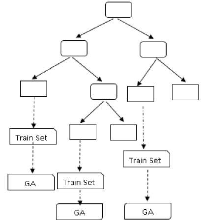
Fig.7. GA small Representation

• d.    Individual Encoding (Rule Encoding)

This is the base step of genetic algorithm, in this phase of the genetic algorithm the chromosomes are represented in the some form so that the they can easily be crossover and muted or they can used in the further operations. The discovered rule by the C4.5 decision tree algorithm are in the form of

IF (condition)tℎen predicted class label

Here condition is called antecedent and the then part of the rule is called the consequent. Discovered C4.5 rules are expressed in the disjunctive normal form and each rule condition are in the conjunctive normal form. The antecedent of the rule consists of the n variables i.e. the n number of the conditions. It’s because the all the rules are not necessarily of the same size. So here necessary to fix the size of the minimum and maximum no. of the rule in the antecedent of the discovered rule. The minimum number of rule and the maximum number of the rule is the number of the attributes in the data set. A chromosomes is the set of n genes in genetic, Here chromosomes have n genes and each gene correspond to the one attribute so maximum number of gene in a chromosomes is the number of the predictor attribute in the dataset. First gene of the chromosomes represent the first attribute, second represent the second attribute and the nth gene is correspond to the nth attribute of the dataset. Every gene is attribute value pair and in the encoding each gene is divided into three sub fields namely attribute, operator and the value. The form of the each gene is given below figure 8:

Fig.8. Gene format

Here i = 1,2,3……..   , A( is the ith attribute of the dataset, 0[ is the operator associated with the attribute A( is logical or relational and finally V[j is the jth value of domain of the attribute A[ . In between the genes of the chromosomes an extra field is added that is B[ this represent the active bit it tells whether the gene is active or not. It takes 0 or 1, if its sets to 0 means the rule condition is not active and 1 means rule condition is active. The general structure of the genome is shown below that contains n gene in figure 9:

[]±OPjy^JJ][[£^jA^

Fig.9. Structure of the Genome

For Example the i ^th rule condition “protocol_type= tcp” is transformed into the genome is: here attribute A[ is the “protocol_type”, operator O_t is “=” and the value of the domain of the attribute Vjj is the “tcp”. Let’s take another example rule condition is “byte transfer>145” that could be encoded as attribute A( is the “byte_transfer”, operator 0[ is “>” and the value of the domain of the attribute Vjj is the “145”. The operator “=”is taken because the type of the attribute is categorical and the operator “>” is taken because the attribute type is continuous.

The above encoding of the genome is adaptable w.r.t. the length of the discovered rule or the size of the rule. The earlier encoding of the genome are cope with the fixed length rule. In our method the each genome have the fixed size and is depends on the value of the A( in such a way individual rule have the variable length i.e. The different individual have the different number of rule condition.

• e.    Selection

This is the most important step in the genetic algorithm, in this step individual genome is selected from the universe of the population for the generation of the new population from the parents. The general procedure for the selection of parents is as given below:

• 1.    Fitness evaluation of each individual.

• 2.    Sorting of the individual in descending order according to the fitness value calculated in the previous.

• 3.    Select the n individuals which have the highest fitness value.

These steps are repeated until best individuals are not found. There are different methods available for selection like roulette-wheel selection, tournament selection etc. In our intrusion detection we used tournament selection method for selection of individual or genome and the size of the tournament is 2. Tournament selection in genetic algorithm is a method to select individual genomes from the population as a possible solution and then it is further used for generation. In this method the tournaments among the genome is carried out between the randomly selected individuals from the population. The winner of each tournament is selected for the generation of the new population from the parents. The winner is removed from the population otherwise one individual may select more than once. The motivation behind selection of tournament method as a selection method in our intrusion detection system is easy to use, it’s also parallel architectures and the most important is it is fair selection method in other words it easily handle the selection pressure.

• f.    Crossover

Crossover mechanism is used in genetic algorithm to generate the next generation of individuals another way we can say that this is the reproduction method. In crossover operation childs are produced from parents. There are different methods available like one point crossover, two point crossover etc. In our intrusion detection we used one point crossover with 80% probability or crossover probability. The mutation operation is shown below in the figure 10.

| (Mbytes<3.5(1) | seivice = telnet(l)    ”siv diff host iate < 0.28(1) | fl^ = SF(1)    |

| dst bytes > 3.5(0) | seivice =private(l) | siv diff host late <0.3(1) |fl^ = SH(l) |

(a) Parentbefore crossover)

| dst bytes < 3.5(1) | seivice = tehet(l)    |~siv diff host rate < 0.3(1) |fl^ = SH(l)    |

| dst bytes >3.5(0)   | seivice =private(l) | siv diff host rate < 0.28(1) |fl^ = SF(l) |

Fig.10.Crossover (One point) of individual

The one point cross over is shown in the above figure, where the one point crossover is shown using the | sign, which in between the gene second and gene third of individual genome. Here in figure above genome is built using the four gene attributes are dst_bytes, service, srv_diff_host_rate and flag. Operators are >, < and =.

Attribute domain are 3.5, 4.5 for attribute dst_bytes, telnet, private for attribute service, 0.3 and 0.28 for attribute service, srv_diff_host_rate and the SH, SF for attribute flag. In each gene of individual of parent and offspring the number 1 and 0 within parenthesis denotes the active bit. It is very important to note that the point of crossover is always between the genes not in gene hence the when crossover operation is performed the rule between the parents are swapped as shown in above figure.

• g.    Mutation

The Mutation operation is applied on the gene produced from the parents to maintain the genetic diversity in the solution space or population, to the next generation otherwise may get the same type of child from the two same parent. In the universe we know the each child have some different property from their parents. In other words we can say that the mutation changes the one or more gene values in the genome from its original value which is got after crossover operation and after the mutation operation may the new genome may change wholly from the previous genome, Hence new genome may provide the better solution. The mutation is depends on the user defined mutation probability, the value of the mutation probability is always set to low, if it is high the search will be random search. In our intrusion detection method we set the mutation probability with 1% and further the elitism with an elitist reproduction factor 1 and the best genome in each iteration is passed as it is to the next iteration or generation without alteration. Basically the new rule is produced by the mutation genetic operation, which will take places the attribute value in the mutation operation in the value of the attribute with newly randomly generated value from the domain of the corresponding attribute. The mutation operation is shown below in the figure 11-12:

| dst bytes-< 3.5(1) | service = telna(l) | srv diff hcist rae< 0.3(1) | flag= SH(1) | (a)

| dst tytes>3.5(0) | service-privae(l) | srv diff host rate< 0.28(1) | flag-SF(1) | (b)

Fig.11. Genome (before mutation)

The domain of the attribute flag {SH, SF, S3, S0, RSTO….etc.} here condition in gene (a) is “flag=SH” is and “flag = SF” for the genome (b). The mutation may alter this condition may “flag=S3” and “flag=S0” from the genome (a) and (b) respectively. The genome after mutation shown below in the figure:

| dst b/tes< 3.5(1) | service = telna(l) | srv diff hcist rae<0.3(l)   | flag=S3(l) ]

I a)

| dst bytes >3.5(0) | service = privae(l) | srv diff host rae <0.28(1) | flag=S0(l) |

Fig.12. Genome (after mutation)

• h.    Rule Pruning

Rule pruning operation is used to find the rule that have the small number of rule and the rule have the more gain in the population. In this proposed intrusion detection system a rule pruning procedure is applied to improve the discovered rule after genetic operations. The motivation behind this is to remove such conditions from the antecedent those who have the low impact in the classification procedure to reduce the size of the rule. Due to this act the size of the rule became low and at the same time will take lesser time in the classification process and doesn’t affect the classification performance. The idea of rule pruning is based on the information theoretic concept. The main theme of the this rule pruning method is remove such antecedent from the rule which have the low information gain in the population and keep those rules of the antecedent which have the have information gain. In this way the discovered rule are became more compact and optimized. The rule pruning operation is applied iteratively to all the discovered rule through genetic operations.

For pruning first calculate the information gain of the each condition of the rule and conditions are sorted according to the information gain low to high also not down the sequence of the sorted sequence. In the First step of rule pruning the lowest information gain or the first sorted sequence number is considered for rule pruning whether the condition is kept in the rule or not for this randomly generate a number in between zero and one and is compared with the information gain of the lowest information gain, if it is satisfies then the condition is kept in the rule otherwise condition is removed from the rule .i.e. set the active bit of the condition to zero. This process will repeated until the number of active bit in the rule is not lesser than the minimum number of condition in the rule .i.e. 2 and the iteration is less than the number of attribute in the dataset.

The gain of the ( Ai Opt Vij ) orcondt is calculated using the given below formula in equation (9):

InfoGctin(condt)=info (G)-info (    )(9)

Where, Info (G)=-∑^^1092?, info ()= xcoiid.^

-    ^{∑     | c}di ^{|       |} СЦ | _- | | _∑     | cy ^{|       |} 52 ^|

|    |                      |      |                      |      |               |    |                        |      |                     ||

Here condt is the i ^th condition of the rule, G is the target class, m is the number of classes, Pj is the probability of the number of classes satisfying the j ^th value of the class G in the population. | C[ | is the number instances that satisfies the condt . | ^cij | Is the number of instances that satisfies both condt and j ^th value of the class G. | Ct | is the number of instances that don’t satisfy condt . | ^cij | Is the number of instances that do not satisfy the cond_t and j ^th value of the class G. T is the total number of training examples.

• i.    Fitness Function

The fitness function is used to measure the quality of the rule or evaluate the each solution of the search space and it controls the selection process in the next generation

Here fitness function used combines the two well-known data mining performance parameters that are sensitivity and specificity. The sensitivity is defined as the ratio of the

TP (true positive) and the sum of the TP (true positive) and FN (false negative). i.e.

TP

=

_Tp + FN

Specificity is defined as the ratio of the TN (true negative) and sum of the FP (false positive) and TN (true negative).

TN i.e.                   =

"   *        FP+TN

The fitness function used in our system is the product of the sensitivity and the specificity.

Fitness function =             ∗ Specificity

The motivation behind the fitness function is the multiplied these terms sensitivity and specificity to force genetic algorithm to discover best quality rule which have the high specificity and high sensitivity. The parameter TP, FN, FP and TN are the parameters which are used to evaluate the performance of the classifiers, these are the entries in the confusion matrix. Confusion matrix shows the data about predicted and actual class result in the form of matrix. Columns of the confusion matrix represent the actual values and the row represents the predicted values of the instances. The confusion matrix is shown below in the figure 13:

Confusion Matrix		Actual Values
		+	-
Predicted Values	+	TP(true positive)	FP(False Positive)
	-	FN(False Negative)	TN(True Negative)

Fig.13. Confusion Matrix

Here the confusion matrix shows two class problems one class is “+” and the second one is “-”.

• •    TP (True Positive): Positive are predicted as positive outcome.

• • TN (True Negative): negative are predictedas

negative outcome.

• • FP (False Positive): Negative are predictedas

positive outcome.

• • FN (False negative): positive are predictedas

negative outcome.

• A.    Architecture

  

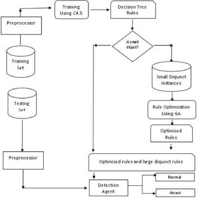
  Fig.14. Architecture DTGA based IDS

  
  
  

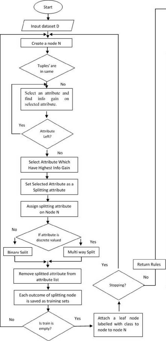
  Fig.15. Flowchart DTGA based IDS

  
  
  

  Input Small Disjunct rule by C4.5

  
  
  
  
  
  
  
  

  Select two parent from based on TSM and increment gen

  
  

  Encode parents based on encoding rule

  
  

  Apply Crossover and mutation based on CP and MP to produce two offspring

  
  

  Decode each offspring

  

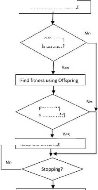
  Offspring distinct?

  Fitness (N)

  Witness (old)

  
  

  Keep the offspring

  
  

  Rule Pruning

  
  
  

  Return Optimized rule and the large disjunct rule

  
  
  

• B.    Pseudo code

Input:

Train: Training Set,

Test: Test Set,

A: attribute list,

AS: attribute selection method,

Max: Maximum Generation,

CP: Crossover Probability,

MP: Mutation Probability,

TSM: Tournament selection method,

T: Threshold for small disjunct,

SD: Small disjunct Training Set

Output:

C4.5 Large Disjunct Rules and GA Optimized Rules

Method:

Step 1. Load the dataset.

Step 2. Create a node N,

Step 3. If tuples in Train are in same class C then return N as a leaf node labelled with class C.

Step 4. For each attribute a in training set.

Step 4.1. Find the information gain ratio from splitting on a according to the subsection (e) of subsection A of the section II.

Step 5. Find the splitting attribute which have the highest information gain ratio from step 4.

Step 6. Label node with splitting criterion;

Step 7. If Splitting attribute is discrete valued then multi-way split allowed then AL=AL- splitting attribute.

Step 8. For each outcome j of splitting criterion (partition the tuples and grows sub tree for each partition) Step 8.1. Let Train j be the set of data tuples in the Train satisfying the outcome j;

Step 8.2. If Train j is empty then attach a leaf labelled with class in D to node N; else attach the node returned by generate_decision_tree (Train j , AS) to node N.

Step 8.3. End for.

Step 9. Repeat step 4 to 8 in each Train j .

Step 10. Generate decision rules from the decision tree created from the above steps.

Step 11. Find the coverage of the each rule in the Train.

Step 11.1. If Coverage of the each rule is less than the threshold T add to the small disjunct SD i ; else add to the rule set R.

Step 12. Randomly select two parents from the i ^th small disjunct which have the same class using the TSM.

Step 13. Do the crossover and mutation based on CP and MP to generate two new offspring.

Step 14. Increment generation i.e. Gen=Gen+1.

Step 15. Repeat for each offspring O i

Step 15.1. Decode offspring O i

Step 15.2. If O i is duplicate in the small disjunct in the SD i then discard it and goto step 16 else compute fitness of the Oi

Step 15.3. If Fitness of Oi is not better than its Parent P i then goto step 16. Else Calculate the overall fitness of the small disjunct from SD .

Step 15.4. If the accuracy of the small disjunct SD is better; than replace Oi with Pi else discard

Step 16. If Gen

Step 17. If there exist any small disjunct go to step 12

Step 18. Prune rule according to the rule pruning method given in the subsection (v) of subsection B of section II.

Step 19. Return optimized rule and the C 4.5 large disjunct rule.

Step 20. Apply Test set on the DTGA based IDS to test the effectiveness.

Step 21. Calculate the performance parameter value

Step 22. Stop

• C.    Flowchart of DTGA based IDS

• IV.    Experimental Result and Discussion

In this subsection we discuss the experimental results and the analysis of the various preliminaries of the experimental process and the classification of the network traffic. The above decision tree and the genetic algorithm based method is used to build a classification. Then the learned model is used to label the unlabeled data instance of the testing set. The process of intrusion detection is very promising field it’s because the computer network is the today one of the basic need of the human being but some ill intended guys coined the terms like hackers, crackers, virus, worms etc. There is no hard and fast rule to detect intrusion in the computer network. Using the historical data to build a classification model to detect the intrusions in the computer network. There are two phases in the model implementation first is training and second is testing. Training phase is used to train the model and testing phase used to label the upcoming network traffic. For training here we used kdd cup data set, the detailed of the kdd cup data set is discussed in the next subsection.

• A.    Dataset

KDD’99 is the most widely used data set for the anomaly detection methods, it contains around 2 million records in test data and approximately 4,900,000 records in training dataset, each of which contains 41 features and one decision attribute. The dataset is prepared by the MIT Lincoln Laboratory. Each network traffic connection is labeled and the dataset contains the five categories of the network attack namely DoS (denial of services), U2R (user to root), R2L (Root to local) and the probe and the total 24 attacks types data are included in the dataset. In other words we can say that the dataset 24 attack types are categorized in the four categories i.e. are DoS, U2R, R2L and probe. The data set contains the 41 attribute and one decision attribute that is class attribute. The class attribute of the dataset depict the whether the connection is normal connection or the anomalous connection. The 41 attributes of the datasets are categorized in four categories basic TCP/IP features, content features and the traffic feature. The basic feature include the basic TCP/IP packet features, content feature are based on the domain knowledge of the connection and the traffic feature includes the connection evaluated in the 2s time frame. Table 5 shows the attribute description and the table 6

Table 5. Dataset features Description

Attribute	Description	Type
duration	duration (number of seconds) of the connection	Numeric
protocol_type	type of the protocol, e.g. tcp, udp, etc.	Nominal
service	network service on the destination, e.g. http, telnet, etc.	Nominal
src_bytes	number of data bytes from source to destination	Numeric
dst_bytes	number of data bytes from destination to source	Numeric
flag	Normal or error flag status of the connection	Nominal
land	1 if connection is from/to the same host/port; 0 otherwise	Numeric
wrong_fragment	number of ``wrong'' fragments	Numeric
urgent	number of urgent packets	Numeric
hot	number of ``hot'' indicators	Numeric
num_failed_logins	number of failed login attempts	Numeric
logged_in	1 if successfully logged in; 0 otherwise	Numeric
num_compromised	number of ``compromised'' conditions	Numeric
root_shell	1 if root shell is obtained; 0 otherwise	Numeric
su_attempted	1 if ``su root'' command attempted; 0 otherwise	Numeric
num_root	number of ``root'' accesses	Numeric
num_file_creations	number of file creation operations	Numeric
num_shells	number of logins of normal users	Numeric
num_access_files	number of operations on access control files	Numeric
num_outbound_cmds	number of outbound commands in an ftp session	Numeric
is_host_login	1 if the login belongs to the ``hot'' list; 0 otherwise	numeric
is_guest_login	1 if the login is a ``guest''login; 0 otherwise	Numeric
count	number of connections to the same host as the current connection in the past two seconds	Numeric
srv_count	sum of connections to the same destination port number	Numeric
serror_rate	% of connections that have ``SYN'' errors	Numeric
rerror_rate	% of connections that have ``REJ'' errors	Numeric
same_srv_rate	% of connections to the same service	Numeric
diff_srv_rate	% of connections to different services	Numeric
srv_serror_rate	% of connections that have ``SYN'' errors	Numeric
srv_rerror_rate	% of connections that have ``REJ'' errors	Numeric
srv_diff_host_rate	% of connections to different hosts	Numeric
dst_host_count	sum of connections to the same destination IP address	Numeric
dst_host_srv_count	sum of connections to the same destination port number	Numeric
dst_host_same_srv_rate	% of connections that were to the same service, among the connections aggregated in dst_host_count	Numeric
dst_host_diff_srv_rate	% of connections that were to different services, among the connections aggregated in dst_host_count	Numeric
dst_host_same_src_port_rate	% of connections that were to the same source port, among the connections aggregated in dst_host_srv_count	Numeric
dst_host_srv_diff_host_rate	% of connections that were to different destination machines, among the connections aggregated in dst_host_srv_count	Numeric
dst_host_serror_rate	% of connections that have activated the flag s0, s1, s2 or s3, among the connections aggregated in dst_host_count	Numeric
dst_host_srv_serror_rate	% of connections that have activated the flag s0, s1, s2 or s3, among the connections aggregated in dst_host_srv_count	Numeric
dst_host_rerror_rate	% of connections that have activated the flag REJ, among the connections aggregated in dst_host_count	Numeric
dst_host_srv_rerror_rate	% of connections that have activated the flag REJ, among the connections aggregated in dst_host_srv_count	Numeric
class	Type of attacks	Nominal

Table 6. Dataset statistics for experiment

Dataset	Training Samples	Testing Samples
Sample 1	202896	22544
Sample 2	106650	11850
Sample 3	226728	25192

• B.    Performance Parameters

The performance parameters specifies the qualities of the proposed model, in other words we can say that the performance parameters specifies the strength and weakness of the model. Here we used the classification accuracy and classification error as a performance parameters. The classification accuracy depicts the how much instances model can correctly classified and the classification error depicts the how much instances model can incorrectly classified, both the parameters are expressed in terms of percentage.

:

Correctly Classified Instances Total Number of Instances

X 100

:

Incorrectly Classified Instances Total Number of Instances

X 100

C. Result

Table 7. Results of proposed model with data sample1

	Accuracy	Error
T=5	99.2705406900	0.7294593100
T=10	99.3114699600	0.6885300400
T=15	98.2015771300	1.7984228700
T=20	99.3100049300	0.6899950700
DT	96.9282700400	3.0717299600

Table 8. Results of proposed model with data sample2

	Accuracy	Error
T=5	97.9746835400	2.0253164600
T=10	98.1200187500	1.8799812500
T=15	98.3309892200	1.6690107800
T=20	96.0872011300	3.9127988700
DT	94.8194861700	5.1805138300

Table 9. Results of proposed model with data sample2

	Accuracy	Error
T=5	99.7860873700	0.2139126300
T=10	99.3114699600	0.6885300400
T=15	99.8907103800	0.1092896200
T=20	99.0114699600	0.9885300400
DT	98.6603800700	1.3396199300

D. Discussion

In this section we presented the discussion of the results of the proposed decision tree and the genetic algorithm based intrusion detection system (DTGA IDS). Figure 14-15 shows the architecture and the flow chart of the system. To evaluate the performance of the system we applied the 3 samples of the kdd cup data set. The dataset is standard dataset designed by DARPA, each samples taken for experimental work are preprocessed to remove the outliers using the interquartile range. The training dataset is used to train the model and then the testing dataset is used to evaluate the performance and the results are recorded on the table given on the result section. The proposed model is implemented on the windows 8, 4 GB Ram, java 1.8 environment, keel and weka. The decision tree C4.5 is used to generate the rule set and the rules those who falls in the category of the small disjuncts are optimized and pruned with the help of the genetic algorithm. The DTGA based IDS uses the threshold 5, 10, 15 and 20 to check the rule generated by the decision tree is whether small disjunct or not. If the rule generated is fall in the small disjuncts category then the leafs training samples are considered as the small disjunct training set and then evaluate the rule on this sample to optimize the rule using the genetic operations crossover and the mutations. The crossover and the mutation probability are 80 percent and the 1 percent respectively. The DTGA based IDS is tested on the different generation value for the genetic evolution 100,150, 200 and 250 generation and the records are here presented are best value at the 200 generations. The quality of the model evaluated with the help of the classification accuracy and the classification error. The table 7, 8, 9 and 10 depicts the results of the model presented in this paper and also the comparative study with the some well-known intrusion detection system. Table 7 shows the results of the sample 1 and table 8 shows the results of the sample 2, table 9

Table 10. Performance comparison of proposed model with different existing model

	Accuracy	Error
C45 (sample 1)	96.9282700400	3.0717299600
C45 (sample 2)	94.8194861700	5.1805138300
C45 (sample 3)	98.6603800700	1.3396199300
*Proposed (T=5)	99.7860873700	0.2139126300
*Proposed(T=10)	99.3114699600	0.6885300400
*Proposed(T=15)	99.8907103800	0.1092896200
*Proposed(T=20)	99.3100049300	0.6899950700
Naive Bayes[20]	92.2700000000	7.7300000000
Rep Tree[20]	89.1100000000	10.8900000000
Random Tree[20]	88.9800000000	11.0200000000
Random forest[20]	89.2100000000	10.7900000000
DTLW IDS[20]	98.3800000000	1.6200000000

*best result at threshold level shows the results of the sample 3 and the table 10 shows the comparative study of the proposed model with the C4.5, Random Tree, Naïve Bayes, DTLW IDS and Reptree. Table 7 shows the result of the sample 1 of the C4.5 and the DTGA small at the threshold level 5, 10, 15 and 20. We can see that the our proposed model provide the best accuracy at the threshold level 10 that is 99.3114699600 and at the same level it provides the 0.6885300400 percent false alarm and the second best result at the threshold level 20 that is the 99.3100049300 accuracy and the error 0.6899950700 percent. C4.5 decision tree method gives the accuracy 96.9282700400 and the 3.0717299600 error on the sample 1 of the kddcup dataset. One of the important observation notable here is the DTGA based IDS here performed very well at all the threshold level.

Table 8 shows the result of the sample 2 of the C4.5 and the DTGA small at the threshold level 5, 10, 15 and 20. We can see that the our proposed model provide the best accuracy at the threshold level 15 that is 98.3309892200 and at the same level it provides the 1.6690107800 percent false alarm and the second best result at the threshold level 10 that is the 98.1200187500 accuracy and the error 1.8799812500 percent. C4.5 decision tree method gives the accuracy 94.8194861700 and the 5.1805138300 error on the sample 2 of the kddcup dataset.

Table 9 shows the result of the sample 3 of the C4.5 and the DTGA small at the threshold level 5, 10, 15 and 20. We can see that the our proposed model provide the best accuracy at the threshold level 15 that is 99.8907103800 and at the same level it provides the 0.1092896200 percent false alarm and the second best result at the threshold level 5 that is the 99.7860873700 accuracy and the error 0.2139126300 percent. C4.5 decision tree method gives the accuracy 98.6603800700 and the 1.3396199300 error on the sample 3 of the kddcup dataset.

Table 10 shows the comparative study of the proposed model with the other systems REP Tree, Random Tree, Random Forest, Naïve Bayes, DTLW IDS and the C4.5 decision tree methods. In this paper the DTGA based IDS best value at each 5, 10, 15 and 20 threshold level are taken. The table shows that our method provide the best result in terms of the classification accuracy and the classification error and the results are expressed in terms of the percentage. The best classification accuracy of the our model is 99.8907103800 and the error is 0.1092896200 at the threshold level 15 and the second best result is 99.7860873700 and the error is 0.2139126300 at the threshold level 5.

• V.    Conclusion

Intrusion detection system are used for the network monitoring to detect the suspicions packets in the computer network whether it is private or public. Today’s IDS system faces the problem of high false alarm rate in the network environment. Decision tree is the very important non parametric classifier. It is easy to implement and also it provide the high accuracy rate but the decision tree is cope with the problem of the small disjunct. In this paper C4.5 decision tree and genetic algorithm based intrusion detection system is proposed. The proposed system solve the problem of small disjunct in the decision tree and also improve the classification accuracy and lowered the false alarm rate. The proposed system is compared with the some well-known system. The Results shows that the proposed system gives better results as compared to the existing systems.